adams路面文件(严选参考)

合集下载

ADAMS路面模型和轮胎UA模型中各全参数含义

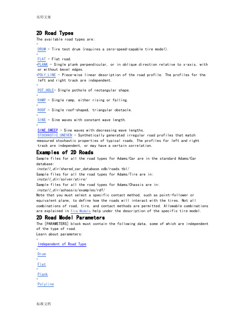
2D Road TypesThe available road types are:•DRUM - Tire test drum (requires a zero-speed-capable tire model). •FLAT - Flat road.•PLANK - Single plank perpendicular, or in oblique direction relative to x-axis, with or without bevel edges. • POLY_LINE - Piece-wise linear description of the road profile. The profiles for the left and right track are independent. •POT_HOLE - Single pothole of rectangular shape. •RAMP - Single ramp, either rising or falling. •ROOF - Single roof-shaped, triangular obstacle. •SINE - Sine waves with constant wave length. •SINE_SWEEP - Sine waves with decreasing wave lengths.•STOCHASTIC_UNEVEN - Synthetically generated irregular road profiles that match measured stochastic properties of typical roads. The profiles for left and right track are independent, or may have a certain correlation. Examples of 2D RoadsSample files for all the road types for Adams/Car are in the standard Adams/Car database:install_dir /shared_car_database.cdb/roads.tbl/Sample files for all the road types for Adams/Tire are in: install_dir /solver/atire/Sample files for all the road types for Adams/Chassis are in: install_dir /achassis/examples/rdf/Note that you must select a specific contact method, such as point-follower or equivalent plane, to define how the roads will interact with the tires. Not allcombinations of road, tire, and contact methods are permitted. Allowable combinations are explained in Tire Models help under the description of the specific tire model.2D Road Model ParametersThe [PARAMETERS] block must contain the following data, some of which are independent of the type of road. Learn about parameters:•Independent of Road Type •Drum •Flat •Plank •Polyline•Pothole•Ramp•Roof•Sine•Sweep•Stochastic UnevenParameters Independent of Road TypeThe following parameters are required regardless of the road type.If ROAD_TYPE = drum, then define the following parameters:If ROAD_TYPE = flat, then no further parameters are required.Parameters for Road Type of PlankIf ROAD_TYPE = plank, then define the following parameters:If ROAD_TYPE = poly_line, then the [PARAMETERS] block must have a (XZ_DATA) subblock. The subblock consists of three columns of numerical data:•Column one is a set of x-values in ascending order.•Columns two and three are sets of respective z-values for left and right track.The following is an example of the full [PARAMETERS] Body for a road type of polyline: $---------------------------PARAMETERS[PARAMETERS]OFFSET = 0ROTATION_ANGLE_XY_PLANE = 180$(XZ_DATA)0 0 01000 100 502000 -1000 1003000 -100 1003001 50 04000 -100 100The XZ_DATA subblock can be extremely large. In this case, only the portion that is needed at the moment is loaded. To facilitate efficient reloading while simulation is running, do not use any comment lines in a subblock that contains more than 2000 lines. Parameters for Road Type of PotholeIf ROAD_TYPE = pot_hole, then the parameters are:If ROAD_TYPE = ramp, then the parameters are:If ROAD_TYPE = roof, then the parameters are:If ROAD_TYPE = sine, then the parameters are:amplitude Amplitude of sine wave (a).wave_lengthWave length of sine wave ().start Start of sine waves (traveldistance) (s s).The road height, z, is given by:Parameters for Road Type of Stochastic UnevenA stochastic uneven road profile both for left and right wheels is generated, with properties very close to measured road profiles.In a first step, discrete white noise signals are formed on the basis of nearly uniformly distributed random numbers. Two of these numbers are assigned to every 10 mm of travel path. The distribution of these random numbers is approximated by summing several equally distributed random numbers, taking advantage of the ‘law of large numbers’ of mathematical statistics.Next, these values are integrated with respect to travel distance, using a simplefirst order time-discrete integration filter. The independent variable of that filter is not time, but travel path. That is why the filter cutoff frequency is controlled by a path constant instead of a time constant. The filter process results in two approximate realizations of white velocity noise; that is, two signals, thederivatives of which are close to white noise. Signals with that property are known as road profiles with waviness 2. Several investigations in the past showed that the waviness derived from measured road spectral densities ranges from about 1.8 to 2.2. The last step is to linearly combine the two realizations of the aboveprocess:,, resulting in the left and right profile,. This is done such that the two signals are completely independent if , and identical if:If ROAD_TYPE = stochastic_uneven, then the parameters are:The parameter: Indicates:intensity Variable to control intensity of white velocity noise, whichapproximates measured spectra of road profiles fairly well.path_constant Variable to control high-pass integration filter.correlation_rl Variable to control correlation between left and right track:•If 0, no correlation.•If 1, complete correlation (that is, left track = right track). Can be any value between 0 and 1.startStart of unevenness (travel distance).Parameters for Road Type of SweepIf ROAD_TYPE = sine_sweep, then the parameters are:[PARAMETERS] Data for Road Type of Sine Sweep The parameter: Indicates:start Start of swept sine wave (travel distance) (). endEnd of swept sine wave (travel distance) ().amplitude_at_sta rtAmplitude of swept sine wave at start travel distance (). amplitude_at_end Amplitude of swept sine wave at end travel distance ().wave_length_at_s tartWave length of swept sine wave a start travel distance ().wave_length_at_e ndWave length of swept sine wave at end travel distance. Must be less than or equal to wave_length_at_start ().sweep_type•sweep_type = 0: frequency increases linearly with respect to travel distance. •sweep_type = 1: wave length decreases by a constant factor per cycle. Depending on the value of sweep_type, the road height is given by the following functions, where:• Linear sweep: (sweep_type = 0) The frequency increases linearly with respect to travel distance. The road height value z (s) as function of travel distance s is alculated as follows:Note the factor 2 in the denominator is not an error. The actual frequency (= derivative of the sine function argument with respect to travel path, divided by ; this is not equal to that factor that is multiplied by in the sine function) is given by thefollowing:•Logarithmic sweep: (sweep_type = 1) with every cycle, the wave length decreases by a constant factor. The road height value is calculated as follows:where:is the travel path where theoretically an infinitely high frequency was reached, measured relative to sweep start . Theactual frequency is given by:Using the UA-Tire ModelLearn about using the University of Arizona (UA) tire model:•Background Information •Tire Model Parameters •Force Evaluation •Operating Mode: USE_MODE •Tire Carcass Shape •Property File Format ExampleBackground Information for UA-TireThe University of Arizona tire model was originally developed by Drs. P.E. Nikravesh and G. Gim. Reference documentation: G. Gim, Vehicle Dynamic Simulation with aComprehensive Model for Pneumatic Tires, PhD Thesis, University of Arizona, 1988. The UA-Tire model also includes relaxation effects, both in the longitudinal and lateral direction.The UA-Tire model calculates the forces at the ground contact point as a function of the tire kinematic states, see Inputs and Output of the UA-Tire Model. A description of the inputs longitudinal slip k, side slip a and camber angle can be found in About Tire Kinematic and Force Outputs. The tire deflection and deflection velocity are determined using either a point follower or durability contact model. For more information, see Road Models in Adams/Tire . A description of outputs, longitudinal force Fx, lateral force Fy, normal force Fz, rolling resistance moment My and self aligningmoment Mz is given in About Tire Kinematic and Force Outputs. The required tire model parameters are described in Tire Model Parameters.Inputs and Output of the UA-Tire ModelDefinition of Tire Slip QuantitiesSlip Quantities at Combined Cornering and Braking/TractionThe longitudinal slip velocity Vsx in the SAE-axis system is defined using thelongitudinal speed Vx, the wheel rotational velocity , and the effective rolling radius Re:The lateral slip velocity is equal to the lateral speed in the contact point with respect to the road plane:The practical slip quantities (longitudinal slip) and (slip angle) are calculated with these slip velocities in the contact point:When the UA Tire is used for the force calculation the slip quantities during positive Vsx (driving) are defined as:The rolling speed Vr is determined using the effective rolling radius Re:Note that for realistic tire forces the slip angle is limited to 45 degrees and thelongitudinal slip Ss (= ) in between -1 (locked wheel) and 1.Lagged longitudinal and lateral slip quantities (transient tire behavior)In general, the tire rotational speed and lateral slip will change continuously because of the changing interaction forces in between the tire and the road. Often the tire dynamic response will have an important role on the overall vehicle response. For modeling this so-called transient tire behavior, a first-order system is used both forthe longitudinal slip as the side slip angle, . Considering the tire belt as a stretched string, which is supported to the rim with lateral spring, the lateral deflection of the belt can be estimated (see also reference [1]). The figure below shows a top-view of the string model.Stretched String Model for Transient Tire BehaviorWhen rolling, the first point having contact with the road adheres to the road (no sliding assumed). Therefore, a lateral deflection of the string will arise that depends on the slip angle size and the history of the lateral deflection of previous points having contact with the road.For calculating the lateral deflection v1 of the string in the first point of contact with the road, the following differential equation is valid during braking slip:with the relaxation length in the lateral direction. The turnslip can be neglected at radii larger than 10 m. This differential equation cannot be used at zero speed, but when multiplying with Vx, the equation can be transformed to:When the tire is rolling, the lateral deflection depends on the lateral slip speed; at standstill, the deflection depends on the relaxation length, which is a measure for the lateral stiffness of the tire. Therefore, with this approach, the tire is responding to a slip speed when rolling and behaving like a spring at standstill. When the UA Tire is used for the force calculations, at positive Vsx (traction) the Vx should be replaced by Vr in these differential equations.A similar approach yields the following for the deflection of the string in longitudinal direction:Now the practical slip quantities, ’ and ’, are defined based on the tire deformation:These practical slip quantities and are used instead of the usual and definitions for steady-state tire behavior. kVlow_x and kVlow_y are the damping rates at low speed applied below the LOW_SPEED_THRESHOLD speed. For the LOW_SPEED_DAMPING parameter in the tire property file yields:kVlow_x= 100 · kVlow_y= LOW_SPEED_DAMPINGNote: If the tire property file's REL_LEN_LON or REL_LEN_LAT = 0, then steady-state tire behavior is calculated as tire response on change of the slip and .Tire Model ParametersSymbol: Name in tire propertyfile: Units*: Description:r1 UNLOADED_RADIUS L Tire unloaded radiuskz VERTICAL_STIFFNESS F/L Vertical stiffnesscz VERTICAL_DAMPING FT/L Vertical dampingCr ROLLING_RESISTANCE L Rolling resistance parameter Cs CSLIP F Longitudinal slip stiffness,C CALPHA F/A Cornering stiffness,C CGAMMA F/ACamber stiffness,UMIN UMIN - Minimum friction coefficient(Sg=1)UMAX UMAX - Maximum friction coefficient(Ssg=0)x REL_LEN_LON L Relaxation length inlongitudinal directiony REL_LEN_LAT L Relaxation length in lateraldirection* L=length, F=force, A=angle, T=timeForce Evaluation in UA-Tire•Normal Force•Slip Ratios•Friction CoefficientNormal ForceThe normal force F z is calculated assuming a linear spring (stiffness: k z ) and damper (damping constant c z ), so the next equation holds:If the tire loses contact with the road, the tire deflection and deflection velocity become zero so the resulting normal force F z will also be zero. For very small positive tire deflections the value of the damping constant is reduced and care is taken to ensure that the normal force Fz will not become negative.In stead of the linear vertical tire stiffness cz , also an arbitrary tire deflection - load curve can be defined in the tire property file in the section[DEFLECTION_LOAD_CURVE], see also the Property File Format Example. If a section called [DEFLECTION_LOAD_CURVE] exists, the load deflection datapoints with a cubic spline for inter- and extrapolation are used for the calculation of the vertical force of the tire. Note that you must specify VERTICAL_STIFFNESS in the tire property file but it does not play any role.Slip RatiosFor the calculation of the slip forces and moments a number of slip ratios will be introduced:Longitudinal Slip Ratio: SsThe absolute value of longitudinal slip ratio, Ss, is defined as:Where k is limited to be within the range -1 to 1.Lateral Slip Ratios: Sa , Sg , SagThe lateral slip ratio due to slip angle, S, is defined as:The lateral slip ratio due to inclination angle, S, is defined as:A combined lateral slip ratio due to slip and inclination angles, S, is defined as:where is the length of the contact patch.Comprehensive Slip Ratio: SsagA comprehensive slip ratio due to longitudinal slip, slip angle, and inclination angle may be defined as:Friction CoefficientThe resultant friction coefficient between the tire tread base and the terrain surfaceis determined as a function of the resultant slip ratio (Ss) and friction parameters (UMAX and UMIN ). The friction parameters are experimentally obtained data representing the kinematic property between the surfaces of tire tread and the terrain.A linear relationship between Ss and , the corresponding road-tire friction coefficient, is assumed. The figure below depicts this relationship.Linear Tire-Terrain Friction ModelThis can be analytically described as:m = UMAX - (UMAX - UMIN) * SsagThe friction circle concept allows for different values of longitudinal and lateralfriction coefficients (x and y) but limits the maximum value for both coefficientsto . See the figure below.Friction Circle ConceptThe relationship that defines the friction circle follows:or andwhere:Slip Forces and MomentsTo compute longitudinal force, lateral force, and self-aligning torque in the SAE coordinate system, you must perform a test to determine the precise operating conditions. The conditions of interest are:•Case 1: 0•Case 2: 0 and C S C S•Case 3: 0 and C S C S•Forces and moments at the contact pointThe lateral force Fh can be decomposed into two components: Fha and Fhg. The twocomponents are in the same direction if a· g < 0 and in opposite direction if 0. Case 1. ag < 0Before computing the longitudinal force, the lateral force, and the self-aligning torque, some slip parameters and a modified lateral friction coefficient should bedetermined. If a slip ratio due to the critical inclination angle is denoted by S c, then it can be evaluated as:If Ssc represents a slip ratio due to the critical (longitudinal) slip ratio, then it can be evaluated as:If a slip ratio due to the critical slip angle is denoted by S c, then it can be determined as:when Ss Ssc.The term critical stands for the maximum value which allows an elastic deformation of a tire during pure slip due to pure slip ratio, slip angle, or inclination angle. Whenever any slip ratio becomes greater than its corresponding critical value, an elastic deformation no longer exists, but instead complete sliding state representsthe contact condition between the tire tread base and the terrain surface.A nondimensional slip ratio Sn is determined as:where:A nondimensional contact patch length is determined as:A modified lateral friction coefficient is evaluated as:where is the available friction as determined by the friction circle.To determine the longitudinal force, the lateral force, and the self-aligning torque, consider two subcases separately. The first case is for the elastic deformation state, while the other is for the complete sliding state without any elastic deformation of a tire. These two subcases are distinguished by slip ratios caused by the critical values of the slip ratio, the slip angle, and the inclination angle. Specifically, if all of slip ratios are smaller than those of their corresponding critical values, then there exists an elastic deformation state, otherwise there exists only completesliding state between the tire tread base and the terrain surface.(i) Elastic Deformation State: S S c, Ss Ssc, and S S cIn the elastic deformation state, the longitudinal force F, the lateral force F, and three components of the self-aligning torque are written as functions of the elastic stiffness and the slip ratio as well as the normal force and the friction coefficients, such as:where:•is the offset between the wheel plane center and the tire treadbase.•is set to zero if it is negative.•the length of the contact patch.Mz is the portion of the self-aligning torque generated by the slip angle . Mzsand Mzs are other components of the self-aligning torque produced by thelongitudinal force, which has an offset between the wheel center plane and the tire tread base, due to the slip angle and the inclination angle , respectively. The self-aligning torque Mz is determined as combinations of Mz, Mzs and Mzs.(ii) Complete Sliding State: S S c, Ss Ssc, and S S cIn the complete sliding state, the longitudinal force, the lateral force, and three components of the self-aligning torque are determined as functions of the normal force and the friction coefficients without any elastic stiffness and slip ratio as:Case 2:0 and C S C SAs in Case 1, a slip ratio due to the critical value of the slip ratio can be obtained as:A slip ratio due to the critical value of the slip angle can be found as:when Ss Ssc.The nondimensional slip ratio Sn, is determined as:where:The nondimensional contact patch length ln is found from the equation ln = 1 - Sn, and the modified lateral friction coefficient is expressed as:For the longitudinal force, the lateral force and the self-aligning torque two subcases should also be considered separately. A slip ratio due to the critical value of the inclination angle is not needed here since the required condition for Case 2,C S C S, replaces the critical condition of the inclination angle.(i) Elastic Deformation State: Ss Ssc and S SacIn the elastic deformation state:(ii) Complete Sliding State: Ss Ssc and S SacCase 3:0 and C S C SSimilar to Cases 1 and 2, slip ratios due to the critical values of the inclination angle and the slip ratio are obtained as:The nondimensional slip ratio Sn, is expressed as:where:For the longitudinal force, the lateral force, and the self-aligning torque, two subcases should also be considered similar to Cases 1 and 2. A slip ratio due to the critical value of the slip angle is not needed here since the required condition forCase 3, C S C S, replaces the critical condition of the slip angle. (i) Elastic Deformation State: S S c and Ss SscIn the elastic deformation state, F and Mz can be written:(ii) Complete Sliding State: S S c and Ss SscIn the complete sliding state, F, F, Mz, Mzs, and Mzs can be determined by using:respectively. The longitudinal force F , the lateral force F, and three componentsof the self-aligning torques, Mz , Mzs , and Mzs , always have positive values, but they can be transformed to have positive or negative values depending on the slip ratio s, the slip angle , and the inclination angle in the SAE coordinate system. Tire Forces and Moments in the SAE Coordinate SystemFor the general formulations of the longitudinal force Fx, lateral force Fy, and self-aligning torque Mz, in the SAE coordinate system, the three possible combinations of the slip ratio, the slip angle, and the inclination angle are also considered. Longitudinal Force:Fx = sin(k) F , for all cases Lateral Force: F y = -sin() F, for cases 1 and 2F y = sin() F , for case 3 Self-aligning Torque:M z = sin() M z - sin() [-sin() M zs + sin()M zs ]Rolling Resistance Moment:My = -Cr Fz, for a forward rolling tire. My = Cr Fz , for a backward rolling tire.Operating Mode: USE_MODEYou can change the behavior of the tire model through the switch USE_MODE in the [MODEL] section of the tire property file.•USE_MODE = 0: Steady-state forces and moments • The tire forces and moments react instantaneously to changes in the tire kinematic states. •USE_MODE = 1: Transient tire behavior • The tire will have a lagged response because of the so-called relaxation length in both longitudinal and lateral direction. See Lagged Longitudinal and Lateral Slip Quantities (transient tire behavior).•The effect of the relaxation lengths will be most pronounced at low forward velocityand/or high excitation frequencies. •USE_MODE = 2: Smoothing of forces and moments on startup of the simulation •When you indicate smoothing by setting the value of use mode in the tire property file, Adams/Tire smooths initial transients in the tire force over the first 0.1seconds of simulation. The longitudinal force, lateral force, and aligning torque are multiplied by a cubic step function of time. (See STEP in the Adams/Solver online help.) Longitudinal Force FLon = S*FLon Lateral Force FLat = S*FLat Aligning Torque Mz = S*MzTire Carcass ShapeYou can optionally supply a tire carcass cross-sectional shape in the tire property file in the [SHAPE] block. The 3D-durability, tire-to-road contact algorithm uses this information when calculating the tire-to-road volume of interference. If you omit the [SHAPE] block from a tire property file, the tire carcass cross-section defaults to the rectangle that the tire radius and width define.You specify the tire carcass shape by entering points in fractions of the tire radius and width. Because Adams/Tire assumes that the tire cross-section is symmetrical about the wheel plane, you only specify points for half the width of the tire. The following apply:•For width, a value of zero (0) lies in the wheel center plane. •For width, a value of one (1) lies in the plane of the side wall. •For radius, a value of one (1) lies on the tread. For example, suppose your tire has a radius of 300 mm and a width of 185 mm and that the tread is joined to the side wall with a fillet of 12.5 mm radius. The tread then begins to curve to meet the side wall at >+/- 80 mm from the wheel center plane. If you define the shape table using six points with four points along the fillet, the resulting table might look like the shape block that is at the end of the property format example (see SHAPE ).Property File Format Example$--------------------------------------------------------MDI_HEADER [MDI_HEADER]FILE_TYPE = 'tir' FILE_VERSION = 2.0 FILE_FORMAT = 'ASCII'(COMMENTS) {comment_string} 'Tire - XXXXXX''Pressure - XXXXXX' 'TestDate - XXXXXX' 'Test tire''New File Format v2.1'$-------------------------------------------------------------units [UNITS] LENGTH= 'meter' FORCE= 'newton'ANGLE= 'rad'MASS= 'kg'TIME= 'sec'$-------------------------------------------------------------model [MODEL]! use mode123! ------------------------------------------! relaxation lengthsX! smoothingX !PROPERTY_FILE_FORMAT= 'UATIRE'USE_MODE= 2$---------------------------------------------------------dimension [DIMENSION]UNLOADED_RADIUS= 0.295WIDTH= 0.195ASPECT_RATIO= 0.55$---------------------------------------------------------parameter [PARAMETER]VERTICAL_STIFFNESS= 190000VERTICAL_DAMPING= 50ROLLING_RESISTANCE= 0.003CSLIP= 80000CALPHA= 60000CGAMMA= 3000UMIN= 0.8UMAX= 1.1REL_LEN_LON= 0.6REL_LEN_LAT= 0.5$-------------------------------------------------------------shape[SHAPE]{radial width}1.0 0.01.0 0.21.0 0.41.0 0.61.0 0.80.9 1.0$---------------------------------------------------------------------load_curve $ For a non-linear tire vertical stiffness (optional)$ Maximum of 100 points[DEFLECTION_LOAD_CURVE]{penfz}0.0000.00.001212.00.002428.00.003648.00.0051100.00.0102300.00.0205000.00.0308100.0。

adams软件文档集合(五)

验评价方法和标准，重复进行了整车稳态、转向回正等几种典型工况的仿真
试验与分析。对比实车试验测试结果，主要参数项的最大仿真误差均控制在
10％以内。对于实车试验测试和仿真试验测试结果均不理想的性能指标，经
过参数调整可以得到比较理想的仿真结果。
13.基于ADAMS的液压破碎机液压系统仿真以ADAMS/Hydraulics为基础，建立液压系统虚拟样机并探讨仿真分析的方法，给出液压破碎机工作装置斗杆液压举升系统虚拟样机的一个分析实例。
22.基于ADAMS的门式起重机动态性能分析.pdf 起重机在高频率启动和制动过程中,必会给机械系统带来强烈的冲击与振动. 根据某型号门式起重机主要的工作性能参数,计算出该型号门式起重机启动和
制动的载荷.在Pro/E中建立三维模型,保存为X_T文件,然后导入到ADAMS中,赋
14.某自卸车转向与悬架干涉的ADAMS校核和优化设计.pdf
汽车设计中通常采用平面作图法校核转向与悬架干涉量,但该方法有一定缺点。结合某自卸车的方案布置,探索运用ADAMS/View软件对转向与悬架干涉量进行校核和优化设计的方法。以车轮跳动引起的转向与悬架干涉量最小为优化
目标,对转向垂臂的布置位置进行了优化,并对制动引起的转向与悬架干涉量
9.基于ADAMS和Simulink联合仿真的主动悬架控制.pdf
为减少车辆控制系统开发周期和成本,以某皮卡车为研究对象,利用
ADAMS/VIEW软件建立了车辆多体动力学模型;基于随机次优控制策略设计了主动悬架控制器,并通过Matlab/Simulink编写了控制算法对其进行联合仿真,通过不断修正控制参数直至得到满意的控制效果。将采用主动悬架系统得到的仿真结果与采用被动悬架系统得到的仿真结果进行了性能对比,结果表明主动悬架系统有效地改善了车辆的行驶性能。

AdamsCar路面谱模型建立以及整车底盘部件载荷提

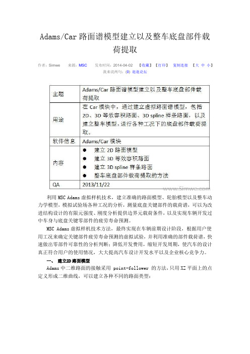
Adams/Car路面谱模型建立以及整车底盘部件载荷提取作者：Simwe 来源：MSC发布时间：2014-04-02 【收藏】【打印】复制连接【大中小】我来说两句：(0) 逛逛论坛利用MSC Adams虚拟样机技术，建立准确的路面模型、轮胎模型以及整车动力学模型，模拟试验场各种工况的分析，测量底盘关键部件的载荷谱，可以为改进结构设计的有限元强度、刚度分析提供边界元载荷条件，以及实现车辆开发过中车身与底盘关键零部件的疲劳寿命预测。

MSC Adams虚拟样机技术方法，最终实现在车辆前期设计阶段，根据用户使用工况来确定关键部件疲劳寿命预测的虚拟试验，并利用准确的部件载荷谱，快速做出零部件可靠性的分析判断；降低开发费用，缩短开发周期，使汽车的设计真正符合用户的使用情况，大大提高汽车设计开发水平以及企业核心竞争力。

一、建立2D路面模型Adams中二维路面的接触采用 point-follower 的方法，只用XZ平面上的点定义形成二维曲线，可以建立各种不同的路面类型：汽车主机厂通常会进行整车跨越三角形凸起路面工况，确认车辆行驶跨越突起路面时的前/后悬架系统、转向系统及车身受冲击受力（上下入力）强度的试验，此时就可以用二维路面描述建立路面模型。

各种不同形状的路面，通过在路面文件中定义各数据块参数完成定义，具体不同路面参数，如下图所示：上一页 1 23下一页二、3D等效容积路面建立3D 等效体积模型为三维的轮胎-路面接触模型，用来计算路面和轮胎之间交叉的体积。

路面是用一系列离散的三角形片来表示，而轮胎则用一系列的圆柱表示。

采用此路面模型，你可以模拟车辆在运动过程中碰到路边台阶、凹坑或在粗糙路面或不规则路面上运动的情形。

3D 等效体积路面模型为一般的三维表面，并用一系列的三角形片表示。

右侧的图表示一个由编号为 1 到 6 的六个节点构成的路表面。

六个节点共构成四个三角形的面单元，分别表示为 A、B、 C 和 D。

Adams软件文档资料集锦续(四)

过给干扰力矩设定阈值来判断碰撞是否发生。在此基础上,通过引入系统误差
的方法对算法进行了改进。最后通过ADAMS及MATLAB进行了仿真与分析,结果
表明算法能够有效地、实时地检测碰撞,并且改进后的算法在阈值设定上更为
简单。
12.基于MSC_fatigue的某轻型客车车架疲劳寿命分析针对某轻型客车杂合车在路试5 000 km时车架出现疲劳裂纹的问题,综合采用多体动力学、有限元和疲劳分析方法对其进行疲劳破坏仿真.在 MSC.Adams/Car中建立该车的多体动力学模型得到其在B级路面的载荷历程,在
他5方向的力作为轮心激励进行整车仿真，分解得到车身接附点的疲劳分析载
荷。本文以某轿车车身载荷分解验证了该技术的工程实用性。
7.机械式挖掘机挖掘轨迹的确定挖掘轨迹是机械式挖掘机挖掘理论研究中的重要内容,铲斗只有沿着合理的挖掘轨迹运动,才可以实现高效和低耗作业.分析了等切削角对数螺旋线轨迹模
型的不足,并在此基础上以工作机构的运动关系为出发点,利用机构运动学理
体动力学模型，分析了重型货车在转向盘转角阶跃输入、转角脉冲输入、转
向回正、稳态回转时的转向响应特性。在整车前期工程设计阶段，对该重型
货车动力学性能参数进行摸底，并为后期优化设计提供指导作用。
11.基于力矩误差的净化机器人碰撞检测技术为了保证净化机器人运行过程中安全性,避免造成较大损失,提出了一种基于力矩误差的净化机器人碰撞检测技术。该方法不需要额外传感器,只需以机器人位移、速度、加速度为输入变量,机器人所受到的干扰力矩为输出变量,通
线性振动模型,并用由伪白噪声法生成的符合实际路面统计特性的伪随机序列
来模拟路面不平度.在此基础上,利用数值算法在时域中对汽车的非线性随机
振动响应进行了计算机仿真计算研究.结果表明,这种方法对研究汽车的非线

基于ADAMS的随机路面不平度建模及参数选择

2.Hefei University of Technology ，Hefei 230009 ，China ） Abstract ：The vertical motions and pitch of vehicle has an effect on the comfort and safety of passengers.The vertical vibration is depends on the road unevenness profiles besides engine excitation.It shows that the road unevenness imitated by Partial Wave Adding Model and compared with national standards.Analysed numbers of harmonic have affection for RMS value of road unevenness.demonstrate that the PSD yields of the random time signal are consistent with the road grades standard.It offers reliable excitation signals for controlling research of vehicle vertical dynamic. Key words ：random vibration ；road unevenness ；harmonic superposition ；Parameters Selection
基于 ADAMS 的随机路面不平度建模及参数选择 / 王俊龙，汪
洋，王吉华
设计·研究

基于ADAMS的汽车脉冲路面仿真

基于ADAMS的汽车脉冲路面仿真宋年秀; 刘亚光; 张丽霞【期刊名称】《《汽车零部件》》【年(卷),期】2019(000)009【总页数】4页(P1-4)【关键词】脉冲路面; 脉冲输入; 平顺性【作者】宋年秀; 刘亚光; 张丽霞【作者单位】青岛理工大学机械与汽车工程学院山东青岛266033【正文语种】中文【中图分类】U270.20 引言汽车在道路上行驶时难免会遇到诸如减速带、凹坑、凸块等各种不平工况，当汽车通过这些障碍时，轮胎传至驾驶员座椅处的振动加速度会发生较大的波动。

为了将这种行驶工况考虑在内，通常情况下采用长为400 mm的三角形单凸块[1]。

根据试验条件不同，脉冲输入可用相应高度的凸块或减速带，而并未对为何使用三角形凸块或是减速带进行阐述。

针对国家标准GB/T 4970-2009[2]所提出的对路面脉冲激励的评价方法进行仿真分析。

首先基于ADAMS/Car，利用某普及型轿车的相关参数，建立包括悬架、车身、轮胎、转向系统在内的整车系统，对各车速下的包括：矩形凸块、斜角凸块、凹坑、减速带在内的6种脉冲输入进行平顺性仿真，并对仿真结果进行分析比较，得到更适宜作为脉冲输入的脉冲轮廓类型。

最后，在脉冲路面的仿真过程中，将随机路面考虑在内，使平顺性仿真更加符合实际工况。

1 整车模型的建立通过对该轿车的测量以及对其相关参数进行查询，得到了整车的主要参数，如表1所示。

在ADAMS/Car中，根据得到的相关参数建立各个子系统的模型，最后将其组装成整车模型并进行平顺性分析。

本文作者选用轿车的前后悬架分别为双横臂独立悬架以及多连杆悬架，对其进行建模得到如图1和图2所示的悬架模型，最终对各子系统进行装配得到如图3所示的轿车整车模型。

表1 整车主要参数参数数值整车整备质量/kg1 360底盘质心高度/mm560质心距前轴距/mm1 125质心距后轴距/mm1 450车身绕横轴转动惯量/(kg·mm2)6.2×108车身绕纵轴转动惯量/(kg·mm2)2.0×108前悬架垂直刚度/(N·mm-1)31前悬架阻尼系数/(N·s·mm-1)2.8后悬架垂直刚度/(N·mm-1)26后悬架阻尼系数/(N·s·mm-1)2.5前轮距/mm1 432后轮距/mm1 220前后轴距/mm2 631轮胎规格225/55R17图1 双横臂独立悬架图2 多连杆悬架图3 整车模型2 脉冲输入仿真2.1 脉冲输入的建立利用ADAMS/Car对汽车通过脉冲路面的振动进行分析时，可以使用插件Road Builder对脉冲路面进行3D建模，也可以使用后缀名为.rdf的TeimOrbit格式路面文件进行2D或3D路面的创建。

ADAMS路面

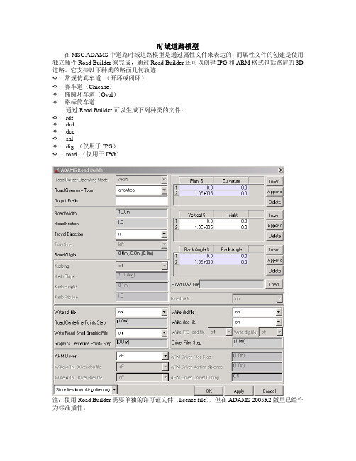
时域道路模型在MSC.ADAMS中道路时域道路模型是通过属性文件来表达的，而属性文件的创建是使用独立插件Road Builder来完成，通过Road Builder还可以创建IPG和ARM格式包括路肩的3D 道路。

它支持以下种类的路面几何轨迹✧常规仿真车道（开环或闭环）✧赛车道（Chicane）✧椭圆环车道（Oval）✧路标筒车道通过Road Builder可以生成下列种类的文件：✧.rdf✧.drd✧.dcd✧.shl✧.dig （仅用于IPG）✧.road （仅用于IPG）注：使用Road Builder需要单独的许可证文件（license file），但在ADAMS 2005R2版里已经作为标准插件。

在ADAMS里路面模型是通过后缀名为.rdf的路面文件引入到仿真环境中，路面文件的结构仍然是TeimOrbit格式的ASCII文本文件。

例如在操纵性仿真中常用的平整路面文件有：在路面文件中的标题数据块、单位数据块的定义方式与DCF、DCD文件一样，[MODEL]数据块定义路面的类型，[GRAPHICS]数据块定义路面几何图形，注意，在2D道路中只有平整路面Flat才有路面图形；其他类型的路面可以通过专用软件包FTire-tools提供的road visualization功能观察路面形状（另一种方法是用函数构造器下的create_shell_from_rdf函数将路面文件转化为shell文件，再将shell壳文件加入到模型中）；[PARAMETERS]数据块定义路面的如摩擦系数、几何形态等参数。

道路类型：道路的类型在TeimOrbit格式的道路属性文件中通过[MODEL]数据块中的METHOD、ROAD_TYPE语句定义，[MODEL]数据块定义的常用道路类型如下：[FUNCTION_NAME]函数名称变量指路面与轮胎接触函数ID 号2D 道路文件MTTHOD ＝2D 时二维路面的参数[PARAMETERS]子数据块：参数子数据块[PARAMETERS]的结构根据路面类型的不同而不同，基本上可以划分为3隔部分：通用参数段、路型参数段和数据组，用符号$分开。

Matlab实现ADAMS三维随机路面建模

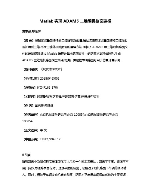
Matlab实现ADAMS三维随机路面建模黄志强;郑旺辉【摘要】根据谐波叠加法得到二维随机路面谱,通过改进的谐波叠加法将二维路面谱扩展到三维,形成三维随机路面谱的建模方法.详解了ADAMS中三维随机路面文件的编制规则,通过Matlab编程计算出路面文件中的路面点高程值阵列,生成ADAMS三维随机路面模型文件,仿真计算过程表明路面可用于仿真计算研究.【期刊名称】《现代防御技术》【年(卷),期】2018(046)003【总页数】6页(P165-170)【关键词】谐波叠加法;路面谱;三维路面;仿真;建模;模型文件【作者】黄志强;郑旺辉【作者单位】北京机械设备研究所,北京100854;北京机械设备研究所,北京100854【正文语种】中文【中图分类】TJ812;N945.120 引言随机路面中激励点的高程值变化可以用另一个词汇来表达：路面不平度。

路面不平度[1]定义为道路表面相对于理想平面的偏离，它描述了随机路面下车辆的振动输入。

同时，相较于车辆发动机等激励源，路面不平度是车辆振动系统的主要振源，在建立车辆系统整车数学或者仿真模型进行平顺性分析时，可以忽略发动机等激励源，而将路面不平度激励作为唯一的激励源施加在车上。

路面不平度通常用来描述路面的起伏程度[1]。

对路面谱的研究首先在于获取路面谱，最直接的方法就是测量，为此，研究者们发明了多种路面谱测量设备。

近年来，随着传感器技术、计算机技术和信号处理技术的飞速发展, 人们对路面不平度的采集、测量和各种试验方法也在不断的更新和改进[1],这一领域已经涌现出了多种测量和试验分析的新方法。

一般按照测量原理的不同可分为直接接触式测量仪和非接触式测量仪(响应式测量仪)等。

国内直接接触式测量仪的典型代表是1979年, 国内长春汽车研究所的赵继海等人发明的拖车式真实路形仪[1], 通过测量拖车上前后轮与拖臂等部件之间的角度变化来获得路面的真实路形。

在对一定道路的测量和分析研究中，学者们发现路面不平度虽然不能够用普通数学函数描述，但是其具有随机、平稳、各态历经的特征[1],这些特征在统计学意义上具有完整的理论描述方法，研究发现路面不平度可以用平稳随机过程理论来分析描述。

AdamsCar路面谱模型建立以及整车底盘部件载荷提

路面是用一系列离散的三角形片来表示，而轮胎则用一系列的圆柱表示。

采用此路面模型，你可以模拟车辆在运动过程中碰到路边台阶、凹坑或在粗糙路面或不规则路面上运动的情形。

3D 等效体积路面模型为一般的三维表面，并用一系列的三角形片表示。

右侧的图表示一个由编号为 1 到 6 的六个节点构成的路表面。

六个节点共构成四个三角形的面单元，分别表示为 A、B、 C 和 D。

ADAMS中三维虚拟路面的实现

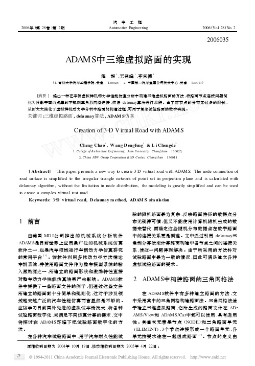
将三维空间点集投影到 X Y 面上 , 得到三维空间散乱点集在 X Y面的二维点集。因为三维空间点集与其在 X Y面上的投影点集之间存在一一对应的关系 ,三维空间点集的三角形连接与其在 X Y 面上的投影点集的三角形连接也存在一一对应的关系 , 因此先将问题简化为二维平面散乱节点的三角剖分 ,再通过数据处理得到三维空间点集的连接关系
[摘要 ] 提出一种在车辆虚拟样机动力学性能仿真分析中构建三维虚拟路面的方法 ,将路面节点连接问题简化为投影平面内点集的不规则三角形网格连接 ,依据 delaunay算法进行求解。由于对节点的分布无过多的限制 , 从而大大简化了虚拟样机动力学分析中路面的构建过程 ,可用于复杂试验路面的数字实现。
2006年 (第 28卷 )第 2期
汽车工程 Automotive Engineering
2006 (Vol. 28) No. 2
2006035
ADAM S中三维虚拟路面的现
程超 1 ,王登峰 1 ,李承德 2
(11吉林大学汽车工程学院 ,长春 130025; 21中国第一汽车集团公司技术中心 ,长春 130011)
图 1 ADAM S软件中路面示意图
根据上述方法 ,用户很容易生成理想的水平路面 ,也可以根据规则分布的节点之间的连接规律 ,编制程序生成一些不太复杂的路面 [ 3 ] 。但在一般情况下 ,复杂路面的节点是随机、杂乱分布的 ,节点之间的连接关系不能用规律性的关系来描述 ,计算无规律分布的离散地面节点的连接关系是路面数字化中的难点。只有解决这一问题 ,建立复杂试验路面才有可能。
( 2) 如果 2个 I ( I = 1, 2)维单形 S1 、S2 ∈T (Ω, V ) ,那么 S1 ∩S2 要么是空集 , 要么是它们公共边或顶点 ,并且是 T (Ω, V )中小于 I维的单形 ;

Adams组合路面的创建方法

Adams组合路面的创建方法Adams/Car提供了方便的2D路面创建工具Road Builder，用户可用该工具创建各类常用路面。

但在做汽车动力学分析时，用户往往需要用到复杂的路面模型，用单一的路面模型不能满足整车分析需要。

这就需要用户根据Adams/Car的路面生成工具进行相对应的路面特征增加，以此来实现多种特征路面的创建。

Adams/Car允许无数个特征的创建，主要应用根据用户需求而定。

1、2D路面创建在Adams/Car中，点击Simulate->Full-Vehicle Analysis->Road Builder，弹出下图所示的路面创建工具。

点击File->Open,在弹出的文件选择框左侧选择mdids：//acar_shared/，在右侧文件夹选择项双击road.tbl，然后选择road_3d_plank_example.rdf。

其他参数不需要更改，主要修改路面的障碍特征即可。

点击Obstacle ，在Obstacle Type 选择pothole ，创建凹坑特征。

凹坑尺寸特征含义如右图所示。

修改Width （坑横向的跨度）为4，length 为0.4，Depth 为0.2，Start Location 改为-5，其他参数不更改。

设定好参数点击Save As ，把路面文件保存为pothole ，所创建路面特征如下图。

2、2D组合创建方法单一特征的路面模型对分析适用性较窄，因此需要创建多种特征组合的路面，来适应分析得需要。

在Adams/Car的Road Builder工具里，可在一个特征的基础上添加多种障碍特征。

保持pothole文件不退出，双击图标进入障碍设定添加项。

在Name空白处输入plank，点击Add，然后双击plank行，退回到特征参数的设定界面。

Obstacle Type改为plank，以下参数分别改为Width 4，Length 0.5，Friction 0.9，Start Location -7，Stop Location -10，Height 0.05，Bevel edge Length 0.002，Plank的参数意义如下图所示。

路面文件

在ADAMS里路面模型是通过后缀名为.rdf的路面文件引入到仿真环境中，路面文件的结构仍然是TeimOrbit格式的ASCII文本文件。

adams软件文档集合(一)

adams软件文档集合(一)
更新时间：2014-11-12
以下是小编整理的一些有关adams软件的系列文档（一）以及文档的简介，其中包括了一些应用案例文档、教程和使用技巧。有关文档的下载，可以到研发埠网站的版块，输入相应的文档名便可查找到。
1.Adams 仿真帮助好奇号探测车实现完美的火星着陆.pdf Adams 仿真帮助好奇号探测车实现完美的火星着陆
7.patran_nastran_adams(update)_solid实例.part2 有关patran_nastran_adams(update)_solid实例
8.ADAMS2012官方培训教程-测量，位移函数和CAD几何.pdf
有关ADAMS2012官方培训教程-测量，位移函数和CAD几何
5.Hypermesh_从nastran到adams的产生柔体几种方法.rar
有关Hypermesh_从nastran到adams的产生柔体几种方法
6.patran_nastran_adams(update)_solid实例.part4 有关patran_nastran_adams(update)_solid实例
、运动空间范围大特点,利用ADAMS规划设计了四足运动步态,并在ADAMS中进
行动力学仿真。仿真分析了对角步态下机器人质心位移、液压缸驱动力以及
与地面的接触力等参数,获得了液压缸工作流量、功率参数。仿真结果验证了
机器人结构设计、步态规划的可行性,为液压缸、发动机选型提供了参考依据
。
14.空气悬架的MATLAB和ADAMS的联合仿真研究
更多资料：/Home.html
19.MSCAdams在方案设计中的使用技巧总结了在方案设计中使用MSC Adams 进行动力学仿真的一些技巧，可有效地提高MSC Adams 软件的使用效率.

(整理)路面ANSYS

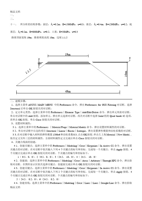
一、二、十一、所分析的结构参数：面层：1h =0.2m ，E=1500MPa ，u=0.3；基层：2h =0.4m ，E=1200MPa ，u=0.2；底基层：3h =0.2m ，E=800MPa ，u=0.2，土基：E=50MPa ，u=0.3 路基顶面宽取19m ，路基填筑高度10m ，边坡1:1.5.2mm二、建模步骤：1、选择主菜单ANSYS MAIN MENU 中的Preferences 命令，弹出Preferences for GUI Filtering 对话框，选择Structural 后单击OK 按钮关闭对话框；2、定义单元类型：选择主菜单中的Preferences ︱Element Type ︱Add/Edit/Delete 命令，弹出单元列表对话框，单击对话框中的Add 按钮，添加单元。

弹出单元选择对话框，再次对话框中选择Solid 组的Quad 4node 42选项，再单击OK 按钮，单击Close 按钮关闭对话框。

3、设置材料属性：3-1、选择主菜单中的Preferences ︱Material Props ︱Material Models 命令，弹出设置材料属性的对话框。

3-2、单击对话框中右边的项目Structural ︱Linear ︱Elastic ︱Isotropic ，弹出设置弹性模量和泊松系数的对话框。

3-3、在对话框中输入材料的弹性模量1500e6和泊松系数0.3，点击OK 按钮。

单击左上角Meterial ︱New Model …依次定义另外三层的材料属性。

全部材料属性定义完成后单击Close 按钮关闭对话框。

4、关键点线面的创建：4-1、创建关键点：选择主菜单中的Preferences ︱Modeling ︱Creat ︱Keypoints ︱In Active CS 命令，弹出设置关键点的对话框。

在对话框中依次输入下列4个关键点的标号和坐标，完成每一个关键点，单击Apply 按钮，4个关键点完成后单击OK 按钮关闭对话框。

汽车平顺性仿真中路面文件生成方法

汽车平顺性仿真中路面文件生成方法
于景飞
【期刊名称】《交通科技与经济》
【年(卷),期】2010(012)006
【摘要】在ADAMS/View中进行汽车平顺性仿真,需要根据不同的实验方法建立相应的路面文件,构造满足仿真要求的路面是该任务的一大难点.探讨在ADAMS仿真中生成各种路面文件的一些方法,生成常用车速下的路面文件,结合整车模型,对生成路面进行验证,仿真结果表明生成方法的可行性及生成路面的正确性.
【总页数】3页(P107-109)
【作者】于景飞
【作者单位】内蒙古科技大学建筑与土木工程学院,内蒙古包头014010
【正文语种】中文
【中图分类】U46
【相关文献】
1.基于ADAMS／Car微型观光电动汽车典型路面平顺性仿真 [J], 乔长胜;李耀刚;琚立颖;冯泽;张文明;
2.碎石路面上汽车平顺性仿真分析 [J], 袁绍华;王昆;王曙光;黄波
3.路面减速带对汽车平顺性和安全性影响的仿真与试验研究 [J], 任成龙;徐慧宝
4.随机路面输入对汽车平顺性的仿真分析 [J], 熊金胜;王天利;张健;章桂林
5.基于虚拟路面的汽车平顺性仿真分析 [J], 刘彪;叶昊;段敏;陈志强;沈澳;郑福民
因版权原因，仅展示原文概要，查看原文内容请购买。

adams路面文件（严选参考）

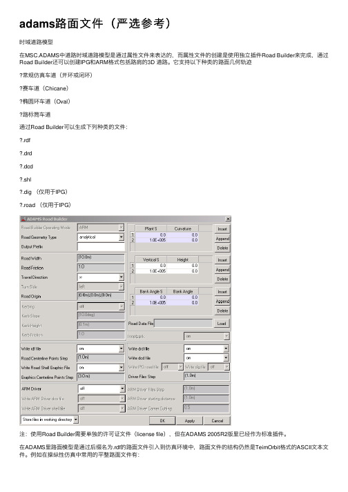
adams路⾯⽂件（严选参考）时域道路模型在MSC.ADAMS中道路时域道路模型是通过属性⽂件来表达的，⽽属性⽂件的创建是使⽤独⽴插件Road Builder来完成，通过Road Builder还可以创建IPG和ARM格式包括路肩的3D 道路。

它⽀持以下种类的路⾯⼏何轨迹常规仿真车道（开环或闭环）赛车道（Chicane）椭圆环车道（Oval）路标筒车道通过Road Builder可以⽣成下列种类的⽂件：.rdf.drd.dcd.shl.dig （仅⽤于IPG）.road （仅⽤于IPG）注：使⽤Road Builder需要单独的许可证⽂件（license file），但在ADAMS 2005R2版⾥已经作为标准插件。

在ADAMS⾥路⾯模型是通过后缀名为.rdf的路⾯⽂件引⼊到仿真环境中，路⾯⽂件的结构仍然是TeimOrbit格式的ASCII⽂本⽂件。

例如在操纵性仿真中常⽤的平整路⾯⽂件有：在路⾯⽂件中的标题数据块、单位数据块的定义⽅式与DCF、DCD⽂件⼀样，[MODEL]数据块定义路⾯的类型，[GRAPHICS]数据块定义路⾯⼏何图形，注意，在2D道路中只有平整路⾯Flat才有路⾯图形；其他类型的路⾯可以通过专⽤软件包FTire-tools提供的road visualization功能观察路⾯形状（另⼀种⽅法是⽤函数构造器下的create_shell_from_rdf函数将路⾯⽂件转化为shell⽂件，再将shell壳⽂件加⼊到模型中）；[PARAMETERS]数据块定义路⾯的如摩擦系数、⼏何形态等参数。

道路类型：道路的类型在TeimOrbit格式的道路属性⽂件中通过[MODEL]数据块中的METHOD、ROAD_TYPE语句定义，[MODEL]数据块定义的常⽤道路类型如下：SINE 正弦波路⾯SINE_SWEEP 正弦变波纹路⾯STOCHASTIC_UNEVEN 随机不平路⾯‘3D’‘ARC904’ /none 3D等效容积道路‘3D_SPLINE’'ARC903'/none 3D样条路⾯'5.2.1' 'ARC913' FLAT或INPUT 521轮胎模型专⽤路⾯‘USER’‘ARC501’⾃定义[FUNCTION_NAME]函数名称变量指路⾯与轮胎接触函数ID号2D道路⽂件MTTHOD＝2D时⼆维路⾯的参数[PARAMETERS]⼦数据块：参数⼦数据块[PARAMETERS]的结构根据路⾯类型的不同⽽不同，基本上可以划分为3隔部分：通⽤参数段、路型参数段和数据组，⽤符号$分开。

ADAMS-Car路面生成技术总结

由此可得到：
2 S （f ） 2 G0u 2 G ( ) 2 2 2
2 1
G ( j )
由此，传递函数 G ( j ) 表达式为：
2
4 2G0u
2
G ( j )
2 G0 u j
因此，路面不平度位移则可以写成时域表达的形式，即为通常所称的积分白噪声形式：
显然，低频长度通常有较大的振幅，而高频短波具有较小的振幅，上图右侧所示的实际路面的频谱密度图就清晰地表明了这一点。国际标准化组织推荐才用路面功率谱密度来描述路面不平度的统计特性，并制订了《机械振动 —道路截面—测量数据报告方法》标准，为单道或多道路面不平度测量数据提供了统一报告方法，适用于乡道、街道、公路以及非路面的不平度测量的数据处理。路面功率谱密度一般采用双对数坐标来描述，通常在高频部分会出现剧烈的波动，因而需要对一定的频带进行光滑处理，用一段或几段直线来表示。其路面功率谱密度光滑计算的频带划分区间如下所示：
S ( n) G0 n p
式中，G0 为路面谱密度不平度系数，其大小随路面的粗糙程度而递增；指数 p 表式双对数坐标下谱密度曲线的斜率。有些情况下，路面谱密度公式包含的斜率可能不连续，这时，则可写成如下形式：
n p1 n nd G0 ( n ) d S ( n) G ( n ) p2 n n 0 d nd
值得注意的是，上述两式中均为空间频率域表达式，与车速无关。如果车辆以恒定的速度在路面上行驶，就可以用时间频率来代替空间频率：
G0u p 1 S( f ) fp
式中， f 为时间频率； u 为车辆行驶速度。对于线性车辆模型来说，上式表示的路面谱可以直接用来作为频域分析的系统输入。然而，如果车辆系统模型中有一些非线性的描述，如双刚度弹簧、非线性阻尼器、限位块撞击等，那么路面模型则必须在时间域或距离域来加以描述。如果得不到实际测量的时间域或距离域信号，通常采用谱密度方程重新“构建”一段路面。因为理论上讲，任意一条路面轨迹均可由一系列离散的正弦波叠加而成。假如已知路面的频域模型，那么每个正弦波的振幅则可由相应频率的频谱密度获得，但相位差则必须由随机数发生器产生。通过这种方法产生的时间域或距离域的路面，便可用于车辆的非线性动力学分析。 2、时域模型

1、下载文档前请自行甄别文档内容的完整性，平台不提供额外的编辑、内容补充、找答案等附加服务。
2、"仅部分预览"的文档,不可在线预览部分如存在完整性等问题,可反馈申请退款(可完整预览的文档不适用该条件!)。
3、如文档侵犯您的权益，请联系客服反馈,我们会尽快为您处理(人工客服工作时间：9:00-18:30)。

时域道路模型
在MSC.ADAMS中道路时域道路模型是通过属性文件来表达的，而属性文件的创建是使用独立插件Road Builder来完成，通过Road Builder还可以创建IPG和ARM格式包括路肩的3D 道路。

它支持以下种类的路面几何轨迹
✧常规仿真车道（开环或闭环）
✧赛车道（Chicane）
✧椭圆环车道（Oval）
✧路标筒车道
通过Road Builder可以生成下列种类的文件：
✧.rdf
✧.drd
✧.dcd
✧.shl
✧.dig （仅用于IPG）
✧.road （仅用于IPG）
注：使用Road Builder需要单独的许可证文件（license file），但在ADAMS 2005R2版里已经作为标准插件。

在ADAMS里路面模型是通过后缀名为.rdf的路面文件引入到仿真环境中，路面文件的结构仍然是TeimOrbit格式的ASCII文本文件。

例如在操纵性仿真中常用的平整路面文件有：
在路面文件中的标题数据块、单位数据块的定义方式与DCF、DCD文件一样，[MODEL]数据块定义路面的类型，[GRAPHICS]数据块定义路面几何图形，注意，在2D道路中只有平整路面Flat才有路面图形；其他类型的路面可以通过专用软件包FTire-tools提供的road visualization功能观察路面形状（另一种方法是用函数构造器下的create_shell_from_rdf函数将路面文件转化为shell文件，再将shell壳文件加入到模型中）；[PARAMETERS]数据块定义路面的如摩擦系数、几何形态等参数。

道路类型：
道路的类型在TeimOrbit格式的道路属性文件中通过[MODEL]数据块中的METHOD、ROAD_TYPE语句定义，[MODEL]数据块定义的常用道路类型如下：
SINE 正弦波路面
SINE_SWEEP 正弦变波纹路面
STOCHASTIC_UNEVEN 随机不平路面
‘3D’‘ARC904’ /none 3D等效容积道路
‘3D_SPLINE’'ARC903'/none 3D样条路面
'5.2.1' 'ARC913' FLAT或INPUT 521轮胎模型专用路面‘USER’‘ARC501’自定义
[FUNCTION_NAME]
函数名称变量指路面与轮胎接触函数ID号
2D道路文件
MTTHOD＝2D时二维路面的参数[PARAMETERS]子数据块：
参数子数据块[PARAMETERS]的结构根据路面类型的不同而不同，基本上可以划分为3隔部分：通用参数段、路型参数段和数据组，用符号$分开。

MTTHOD＝2D时通用参数表
参数描述
offset 参照整车原点的Z向偏移量，默认值＝0
rotation_angle_xy_plane 由于在A/Car中，车辆前进默认的方向是-X方向，路面文件的坐标
系是全局坐标系，所以要将路面文件的x轴翻转，默认为180(deg) mu 道路与轮胎摩擦系数修正比，实际摩擦系数是二者的乘积。

摩擦系
数修正比默认值＝1.0
路型参数段：
ROAD_TYPE ＝FLAT
——平整路面
ROAD_TYPE ＝DRUM
——转鼓试验台
参数子数据块
镶条参数示意图
能可以用ROAD_TYPE ＝plank 代替
ROAD_TYPE = plank —— 凸块路面
参数子数据块
ROAD_TYPE = poly_line —— 折线路面
参数子数据块
HEIGHT
LENGTH
START
[PARAMETERS]必须有(XZ_DATA) 子段；在XZ子段中的3列数据，其意义是：第一列为X值（行程值）；第二列和第三列分别是左右车轮轨迹处的Z向高度。

(XZ_DATA) 子段可以定义得很长（超过200行），且不需要任何注释行，注意折线路面同时定义了两侧的轮辙。

ROAD_TYPE = pot_hole
——凹坑路面
参数子数据块
ROAD_TYPE = ramp
——斜角凸块路面
参数子数据块
ROAD_TYPE = roof ——三角形凸块路面参数子数据块
Height
Start
Length
Depth
Z
X
Start
α
Slope=tan(α)。