优选Ch随机变量序列的极限
Ch8随机变量
Chapter 8 Random Variable8.1 What is a random variable?A random variable (abbreviation: r.v.) assigns a number value to each outcome (simple event, sample point) of a random circumstance. e.g. Toss a die and observe the number of face upRandom variables is denoted by X, Y (or X(ω), when a specific simple eventωis emphasized)●A continuous random variable can takeany value in an interval or a collectionof intervals●A discrete random variable can takeone of a countable list of distinct values 8.2 Discrete random variableExamples1. (Toss a fair coin –the random circumstance)X = the number of times the “head” occurs Then X can take 1(“head”occurs) or 0 (“tail” occurs)2. X = # of defectives in a package of 50 cellphones3. Y = # of calls needed to get through in a fixed time period4. Repeatedly tossing a fair coin, and define the r.v.:X =number of tosses until the head occursThe Probability Distribution of discrete random variablesThe Probability Distribution Function (pdf ) of a discrete r.v. X is a table ,or a rule that assigns probability )(i i x X P p ==to the possible values i x of the r.v. X , denoted by),(~1p 1p 0p p x x X i ii i 1i 1=<<⎪⎪⎭⎫ ⎝⎛∑ The pdf describes completely the probabilistic rule of a discrete r.v.In Example 4, one has P(X =k ) = k21⎪⎭⎫ ⎝⎛, i.e. ⎪⎪⎭⎫ ⎝⎛ k 2121k 1X ~Miniproblem What about tossing a biased coin, where the probability of occurring head is p8.3 Expected value (Mean) for a discrete r.v. Expected value (Expectation ) of a discrete r.v. X , denoted by EX , is a weighted average value of X :i i ip x EX ∑=, which is exactly the Mean value of X , Usually μ is used to represent EX● Describing the central tendency of pdf ● Weighted average of all possible values ● Approximated by the average when the experiment is repeated independently a very large number of timesStandard Deviation for a discrete r.v. Variance of X :i 2i i 2denoteby 2definedby p x EX X E X V )()()(μσ-==-=∑● Weighted average squared deviation fromthe meanStandard Deviation of X : σ=)(X VMeasures the variability of the distributionExample 8.7The randomized schedule I and II are employed respectively for investing $100 Net gains after 1 year for I and for II are⎪⎪⎭⎫ ⎝⎛994005001010005000X 1...$$$~,⎪⎪⎭⎫ ⎝⎛52341020X 2...$$$~. Then10EX EX 21$==,936X V 92172X V 21.$)(,.$)(==Plan II sounds better.8. 4 Binomial Random VariablesBinomial Experiments and Binomial r.v. Binomial Experiment characteristics: ● Sequence of n identical trials● Each trial has 2 outcomes: S(‘Success’) or F(‘failure’)● The probability of success of each trial is p● Trials are independentBinomial r.v.:X = number of S in the n trials Examples⏹# of games Gophers won in the last season ⏹# of defective items in a batch of 5 items ⏹# of correct on a 33 questions quiz ⏹# of customers who purchase out of 100 customers who enter storeThe Probability for Binomial r.v.For a Binomial r.v. X , one hasP (X=k )),()!(!!p 1q n k 0q p k n k n k n k -=≤≤-=-That showsX ~⎪⎪⎭⎫ ⎝⎛--n k n k n p q p k n k n q n k 0 )!(!!, where we say that X has a binomial distribution , and denote it by X ~B(n , p )Microsoft Excel Tips : Calculating P(X=k ) by BINOMDIST(k,n,p,false ) P(X ≤k ) by BINOMDIST(k,n,p,true )(“false ” stands for exactly k successes, “true ” indicates for a cumulative probability)Tendency (Mean) & Standard Deviation of B (n,p ))()(,p 1np X V np EX -==More ExamplesRandom circumstance r.v. distributionToss 3 fair coins, #of H B (3,21)Roll a die 8 times #of 4 or 6 B (8,31)Randomly sample #of seeing B (1000,p ) 1000 US adults UFO p =proportionRoll 2 dies once Sum is 7 B (1, 366)MiniproblemYou t oss 2 coins. You’re interested in the number of tails. What are the expected value & standard deviation of this random variable, number of tails?8.5 Continuous random variables● Infinite number of outcomes in interval, too many to list like discrete variable● Probabilities of taking any special values are 0.ExamplesX = length of time between customer arrivalsSo are height, time, weight, monetary valuesProbability Density FunctionDiffer from determining the probability, we are only able to find the probability that X falls between two values and do this by determining the area between the two values under a curve f(x), called the Probability Density Function of the r.v. X.i.e. f(x) is a probability density function of X, if for any c, d, we have)()(dXcPdXcP<<=≤≤=Area under the curve f(x) between c and df(x) is not probability , but density(密度)hh xXxPxfh )(lim)(+≤≤=→Continuous Random Variable Accumulated Probability Function F(x)=)(XF Area under the curve f(x) between -∞and xExpected value (Mean) and Variance Mean of X :EX =μ = 纵坐标在概率密度函数f (x )与0间,横坐标在),(∞-∞的面积片在横坐标x 处加一个大小为x 的力(如x 值为负, 则表示反向的力), 所得的平衡点的横坐标Variance of X :22EX X E X V σ=-=)()(Standard Deviation of X : σ=)(X V ( 附注 FormulaMean ⎰=dx x xf )(μVariance ⎰-=dx x f x 22)()(μσ )x f x fBasic Rules)()(,)(X V c X V c EX c X E =++=+ )()(,)(X V c cX V cEX cX E 2== StandardizedIf μ=EX , 2X V σ=)( , then0X E =⎪⎭⎫ ⎝⎛-σμ,1X V =⎪⎭⎫ ⎝⎛-σμ where σμ-X is called the Standardized Error of X (随机变量X 对于其均值的无量纲化的随机偏差)Uniform Distribution(均匀分布)If a r.v. X takes equally likely outcomes in interval [c , d ], which is equivalent to that the probability density function f (x ) of X has the form of⎪⎩⎪⎨⎧≤≤-=)()()(otherwise 0d x c if c d 1x f ,then X is said to submit a uniformdistribution on the interval [c , d ], and denoted by X ~U [c , d ]Example 8.13 If you arrive at a bus stop randomly, where the bus comes every 10 minutes. Let X =waiting time until the next bus arrives. Then X ~U [0,10]. The probability that the waiting time between 5 and 7 minutes isP (5 ≤≤X 7) = Base ⨯Height= (7 - 5) 101⨯ = 51Another exampleYou’re the production manager of a soft drink bottling company. You believe that when a machine is set to dispense 12 oz., it really dispenses 11.5 to 12.5 oz. inclusive. Suppose the amount dispensed has a uniform distribution. What is the probability that less than 11.8 oz. is dispensed?Solution: A randomly drawn machine is set to dispense X oz. Then X ~ U [11.5,12.5], andP (11.5 ≤≤X 11.8) = Base ⨯Height = (11.8 - 11.5) ⨯ 1 = 0.30Mean & standard deviation of Uniform r.v.s2d c +=μ,12c d 22)(-=σNormal DistributionProbability Density FunctionWe say that r.v. X submit Normal distribution with parameters2σμ,, if its probability density function has the form off(x) =2x21e21⎪⎭⎫⎝⎛--σμσπ, (0>σ),denoted by X ~N(2σμ,) .The calculation shows that the total area under the above curve is 1.Characters●Mean, median, mode are equal ( =μ)●σis the standard deviation of therandom variable X, which has infinite range, but effective width is 6 σThe area of the following shadow is 0.95 and the area between μ-3σ and μ+3σ is 0.997Effect of Varying Parameters (μ, 2σ)Small 2σ large 2σUsing probability Tables (Reducing to the Standard Normal Distribution N (0,1)) to calculate● If X is a normal r.v. , then aX +b is also anormal r.v. i.e. if),(~2N X σμ, then 22~(,)aX b N a b a μσ++ ● If X ~N (2σμ,), then σμ-X ~N (0,1)(Explain : change mean μ and standard deviation σ into 0 and 1. The value of σμ-=X Z is called z-score in statistics)Numerical Table of function Φ(z ) -- Cumulative Probability Function of the standard Normal Distribution (dx e 21z 2x 21z-∞-⎰=πΦ)() (标准正态分布累积概率函数的数值表: p.538-)(We have 500z 1z .)(),()(=-=-ΦΦΦ)A part of the value of Φ(z)-1/2 is shown asz ):Using z-score to solve problemsExampleP(3.8 ≤ X ≤ 5)= P(0.12 ≤ Z ≤ 0)).()(1200--=ΦΦ0478050120120150..).()].([.=-=--=ΦΦ Example),(~1005N X , then σμ-=X Z and).().().().(210301058Z 10517P 8X 17P ΦΦ-=-≤≤-=≤≤Real exampleYou work in Quality Control for GE. Light bulb life has a normal distribution with mean 2000 hours and standarddeviation 200 hours. What’s the probability that a bulb will last1. between 2000 & 2400 hours?2. less than 1470 hours?477222400X2000P.)()()(=-=≤≤ΦΦ00465216521470XP.).().()(=-=-=≤ΦΦMini-problem 1 (Reliability)Life testing has revealed that a particular type of TV picture tube has a length of life that is approximately normally distributed with a mean of 8000 hours and a standard deviation of 1000 hours. The manufacturer wants to set a guarantee period for the tube that will obligate the manufacturer to replace no more than 5% of all tubes sold. How long should the guarantee period be? Finding Percentiles (百分点)The 25th percentile x of a Normal r.v. isthe value having z-score zσμ-=xsatisfying 250z .)(=Φ. e.g. if the 25th percentile of pulse rate is 64, then there are 25% people has pulse rate below 64.The same way, the p -th percentile x is determined by 100p x =-)(σμΦ Microsoft Excel TipsNORMSDIST(z ) provides )(z ΦNORMSINV(p ) provides z satisfying p z =)(Φ8.7 Approximating Binomial Distribution ProbabilitiesNormal Approximation of a Binomial r.v.:A B (n , p ) r.v. X is approximately to follow the distribution N (np , np (1-p )), i.e. the N (EX , V(X))(Or say, )1(p np npX -- - the standardize of X , isapproximated by the standard normal distribution as n goes to infinite)Example 8.18 Number of Heads in 30 Flips of a fair coin ( B (30, 0.5))The Histogram looks quite like the density function of N (15,7.5)Approximating Cumulative Probabilitiesfor Binomial r.v.s()X np k np k np P X k P ---≤=≤≈ΦPractically, this approximation is applied when both np and n(1-p) are at least 5, and usually at least 10 is preferable8.8 Sums, difference, and Combinations of r.v.A linear combination of r.v. X ,Y ,…means aX+bY+…(including X+Y and X-Y ). ● Rule 1 E (aX+bY+…)=aEX+bEY+… ● Rule 2 If X ,Y ,…are independent , thenV (aX+bY+…)=2a V (X )+ 2b V (Y )+…● Warning: V (-X )(≠-V (X ))=V(X ) Combining Independent Normal r.v.sIf X ,Y are independent, and ),(~2X X N X σμ,),(~2Y Y N Y σμ, then ),(~2Y 2X Y X N Y X σσμμ+++Example (Missing flight or not)Meg leaves home 45 minutes before the last call for her flight will occur. Assume the driving time (minutes) ),(~925N X and the airport time ),(~415N Y , then the probability of missing her flight is))(()(49251545Z P 45Y X P ++->=>+082303911391Z P .).().(=-=>=ΦAdding Binomial r.v.s with the same Success probabilityIf X ,Y are independent, and ),(~p n B X X , ),(~p n B Y Y , then ),(~p n n B Y X Y X ++Example 8.23Strategies for Exam when out of timeTwo-part multiple-choice test with 10 questions in each part and having 4 choices for each question. You need get 13 questions or more right to pass. However, you don ’t have time to study all the materials. Fromexperience you know that if you study all the 20 questions well, then you can narrow all questions into 2 choices. If you study the first part carefully, then you will get right for these questions with probability 0.8, but you have to guess completely the other part. How can you do?Solution: you haveStrategy 1 - Study all the material wellLet S be the scores you will get, then,(=)),S=~,(.,10VS5ES520Ns.d. (standard deviation) =5= 2.24P≤S-=≥=131)((12SP)1- BINOMDIST(12,20,0.5,true) =0.1316 Strategy 2 - Study first part material only Let X and Y be the scores you will get for the part 1 and part 2 respectively, then X and Y are independent and,X.()(=,~=.,),EXX1NV68108(Y.),)(N=~=.,,.VY1105875225EY)(,.+)+=(=VY3475X25XY10E.s.d. of X +Y =473.= 1.86)(13Y X P ≥+is tedious to calculate, since Y X + no more follows the binomial distribution, but )(13Y X P ≥+can be estimated by simulation, which is, e.g. done 1000 times by randomly generating values of X +Y . e.g. there are 130 times of them not smaller than 13. Then we have 13013Y X P .)(≈≥+Conclusion: Neither one looks betterExponential Distribution⎩⎨⎧<≥=-)()()(0x 00x e x f xλλ,denoted by X ~exp λMean: EX =λ1, Variance: V (X ) = 21λConclusion of this chapter● Defined discrete and continuous random variable● Described the binomial, uniform, normal,& exponential random variables●Calculated probabilities for continuous random variable●Exploiting the normal approximation of the binomial distributionExercise of 7th week1. Mini-problem 12. A volunteer organization wants to find donors. 3volunteers agree to call potential donors. In past, about 20%of those called agreed independently to make a donation. If the 3volunteers make 10, 12and 18calls respectively, what is the probability that they get at least 10 donors?3. Alice and Julie each swam a mile a day. Alice’s times are normally distributed with mean =37 minutes and standard deviation =1 minute. Julie is faster but less consistent than Alice, and her times are normally distributed with mean =33minutes andstandard deviation =2 minutes. Their times are independent each other. Can Alice ever win?4. The standard medical treatment for a certain disease is successful in 60% of all cases.(1)The treatment is given to n =200 patients. What is the probability that the treatment is successful for 70% or more of these 200 patients?(2)How about the case of n=205 设),(~p n B X (二项分布).分别对于 12108n ,,=及902010p .,,.,. =,n 10k ,,, =,作出k n k k np 1p C k X P --==)()(的数值表. (若用Matlab ,则要求给出程序与数值表;如用Execel 则要求写出计算的要领与注释(傻瓜化!))6. The number of training units that must be passed before a complex computer software program is mastered varies from one to five, depending on the student. After much experience, the software manufacturer has determined the probability distribution that describes the fraction of usersmastering the software after each number of training units:a. Calculate mean μ, variance σ2, and the standard deviation σ. Interpret μ in the context of the problem.b. Graph p(x). What is the probability that X is in the interval (μ–2σ, μ+2σ )?c. If the firm wants to ensure that at least 70% of the students master the program, what is the minimum number of training units that must be administered?7. A weather forecaster predicts that May rainfall in a local area will be between 3 and 6 cm but has no idea where the amount will be within that interval. Let X be the amount of May rainfall in the local area, and assume that X is uniformly distributed in the interval of 3 to 6 cma. State the density function of X and plot it on a graph.b. Obtain the mean and the standard deviation of the probability distribution.c. What is the probability that the observed Mayrainfall will be less than 5 cm?8. Gauges are used to reject all packages crackerwhere a certain weight is not within the specificationoz. It is know that this weight is normally 225ddistributed with mean 225oz. and variance 441 squareoz. Determine the value d such that the specificationscover 95% of the weight.9. The average life of a certain type of small motor is10 years with standard deviation of 2 years. Assumethat the lifetime of a motor follows a normaldistribution. The manufacturer replaces free allmotors that fail while under guarantee. If he is willingto replace only 3% of the motors that fail, how long aguarantee should he offer?10. The IQs of 600 applicants of a certain college areapproximately normally distributed with a mean of115and a standard deviation of 12. If the collegerequires an IQ at least 95, how many of these studentswill be rejected on this basis regardless of theirqualification?11. The safety jackets produced by a manufacturerhave rating with an average 840newtons(unit of the force) and a standard deviation 15newtons. Suppose that it follows normal distribution. To check whether the process is operating correctly, a manager takes a sample of 100jackets, rates them, and calculates the bar graph, the mean rating for jackets in the sample.(1) What is the probability that the sample mean is less than or equal to 830 newtons?(2) Suppose that on one particular day, the manager observed sample mean = 830. Would you conclude that this indicates that the true process mean for that day is still 840 newtons? Why?。
随机分析1--均方极限

证明
E aX bY
2
E ( a X b Y )( a X b Y )
E ( a X b Y )( a X b Y ) E ( aX
2
bY
2
aX bY aX bY )
aX bY aX bY 2 Re( aX bY )
E a
二阶矩过程的均方微积分
研究对象 一类具有二阶矩的随机过程 研究内容 连续性、可导性与可积性等. 是均方极限意义下的随机微积分
重点
均方极限,均方连续,均方可导
以及均方可积的概念和准则.
要求 掌握均方极限,均方连续,均方可导 以及均方可积的的概念以及相应准则. 熟悉一阶线性随机微分方程及其解. 熟悉正态过程的随机分析的一些结果.
a
k
a l R X ( k , l )收 敛 .
二阶矩过程均方极限定义
设 { X ( t ), t T }是 二 阶 矩 过 程 , X H , t 0 T ,
如 果 lim E X ( t ) X
t t0 2
0,
则 称 当 t t 0时 ,X ( t ), t T }收 敛 于 X . {
定理(均方大数定理)
设 { X n , n 1, 2, } H
是相互独立同分布的随机变量序列,且
E X n , n 1, 2, , 则
l.i.m
n
1
X n
k 1
n
k
,
证明:E
n
1
n i 1
n
1
n
2
Xi
E
2
i 1
(X n
§4.3随机变量序列的两种收敛性

n
再令x ' x F ( x 0) lim Fn ( x )
n
8
同理可证: 当 x " x时,F ( x ") limFn ( x ),
n
再令x " x, F ( x 0) limFn ( x ) .
n
即有 F ( x 0) lim Fn ( x ) lim Fn ( x ) F ( x 0) . n
0, x c; 有 Fn (c / 2) F (c / 2) 1, F ( x ) 1 , x c . Fn (c ) F (c ) = 0 .
从而 P ( X n c ) (n ) 0
且 Fn ( x ) F ( x ) , 所以当 n 时,
n
若x是F ( x )的连续点,
则 Fn ( x ) F ( x ), 即X n X .
W L
TH2表明:依概率收敛是弱收敛的充分不必要条件,
由弱收敛不能得出依概率收敛。见下面的例子。
9
例2 设X
X P
1 1 2
1 1 2
令 Xn X ,
L
当然有 X n X . 则 X n 与X 同分布,
P P P X n a ,Yn b X n Yn a b; P P X n Yn a b , X n Yn a b(b 0). 证明: ( X n Yn ) (a b ) X n a Yn b ( X n Yn ) (a b ) X n a Yn b 2 2
0 P X Y
《概率论与数理统计课件》随机变量序列的收敛性

P
定理 4.3.3 若 C 为常数,则 X n C 的充
L
要条件是 X n C .
21
证明:
必要性已由定理 4.3.2 给出,下证充分性.
记随机变量 X n 的分布函数为 Fn x .而常数 X C
(退化分布)的分布函数为
F
x
0 1
xC . xC
22
所以对于任意的 0 ,有
Fn x收敛到一个极限分布函数 Fx 是有实际意义的.现在的 问题是,如何定义分布函数序列 Fn x的收敛性?很自然,由 于 Fn x是实变量函数序列,我们的一个猜想是:对所有的 x , 要求 Fn x F x, n .这就是数学分析中的点点收敛.然
下面的定理说明了依概率收敛是一种比按分布收敛更 强的收敛性.
11
P
L
定理 4.3.2 如果 X n X ,则必有 X n X .
12
证明:
设随机变量 X n 的分布函数为 Fn x , n 1, 2, 3, ;
随机变量
X
的分布函数为
F x .为证
Xn
L
X
,只须证明:
对所有的 x ,有
写出随机变量 Yn
n k 1
Xk 2k
的特征函数n t ;⑶
证
明:当 n 时,随机变量序列Yn依分布收敛于随机变量Y .
33Leabharlann 解:⑴ 由于随机变量Y 服从区间 1, 1 上的均匀分布,因
此 Y 的特征函数为
t eit eit cost i sin t cost i sin t sin t .
(因为 x x 0).所以有
再令 x x ,得
任意随机变量序列关于广义随机选择系统的若干极限性质
0 引 言
概率论 的极限定理是概率论研究 的基本领域之一. 众所周知 , 对独立随机变量序列 、 马尔可夫链 、 鞅 差序列 的强 大数定 律 已有 了大量 的 研 究 , 得 到 了相 当完 善 的结 果 … . 并 随机 变 换 的概 念 最 早 起 源 于赌
系统 , 献 [ 7 讨 论 了任 意 随机 变 量 序 列 的一 种 特殊 的 随机 变换 ( 文 2— ] 随机 选 择 ) 的强极 限定 理. 本
r t sa e o t ie a i r b an d. o
Ke r s r i a a d m v r b e e u n e;Ma k v p o e s y wo d :a b t r r n o a i l s s q e c ry a r o r c s ;ma t g l i e e c e u n e;r n o r n ae df r n e s q e c i f a d m t n fr ;r n o q i b e r t s t n mi t e r ms r s m a o a d m e u t l ai ;s o g l t h o e a o r i
阶马氏过程 , 鞅序列 , 鞅差序列 , 独立 随机变 量 序列 的一类强极限定理. 把赌博系统的随机变换概 念推 广到任意随机变 量 序列 , 得到 了任意随机变量序列随机选 择 与公 平 比的若 干极 限定理. 关键词 : 任意随机变量序列 ;马氏过程 ; 差 序列 ; 鞅 随机变换 ; 随机公平 比 ; 强极限定理
L n e I j Mi i
(c ol f te ai n hs s J n s i rt o cec n eh o g ,hni g i gu2 2 0 , hn ) Sho o hm tsadP yi ,i guUnv sy f i eadT cnl yZ ej n a s 10 3 C ia Ma c c a e i S n o a Jn
大数定律随机变量序列的收敛定义中心极限定理

>
0.387
?1
F (0.387) = 0.348
16
中心极限定理
例:计算机在进行加法时,对每个加数进行四舍五入取整,设 每个加数相互独立,并均匀分布。若将1500个数相加,误差 总和的绝对值超过15的概率是多少?
D
骣Sn 桫n
?1
C ne2
所以
lim
n
P
禳 镲 镲 睚 镲 镲 铪Sn
-
E(Sn) < e n
=1
7
强大数定律
柯尔莫哥洛夫大数定理:设 X1, X 2 ,... 相互独立,满足
å¥ k=1
D(Xk ) k2
<
?
则
å P
禳 镲 睚 镲 镲 铪nlim
1 n
n(
k=1
X
k
-
E( X k )) = 0
有
lim
n
P
禳 镲 镲 睚 镲 镲 铪fnA
-
p<e
=1
注:伯努利大数定理揭示了随着试验次数增加,频率稳定中心极限定理:设随机变量 X1, X 2 ,... 独立同分
布,且 E( X k ) = m, D( X k ) = s 2, k = 1, 2,...
布,则对于任意 x ,有
lim
n
P 禳 镲 镲 睚 镲 镲 铪
hn - np np(1- p)
?
x
F (x)
15
中心极限定理
例:一加法器同时收到20个噪声电压 Vk (k = 1,..., 20) ,假设 它们相互独立,且都在 (0,10) 上均匀分布,记
求 P{V > 105}
å V =
概率论第十六讲中心极限定理
反查标准正态函数分布表,得
3.09 99.9%
令 解得
a 120
r
3.09
48
a (3.09 48 120)r 141r (千瓦)
例5 设有一批种子,其中良种占1/6. 试估计在任选的6000粒种子中,良种 比例与 1/6 比较上下不超过1%的概率.
Y n ~ N (np , np(1-p)) (近似)
中心极限定理的应用
例1 炮火轰击敌方防御工事 100 次, 每次 轰击命中的炮弹数服从同一分布, 其数学 期望为 2 , 均方差为1.5. 若各次轰击命中 的炮弹数是相互独立的, 求100 次轰击
(1) 至少命中180发炮弹的概率; (2) 命中的炮弹数不到200发的概率.
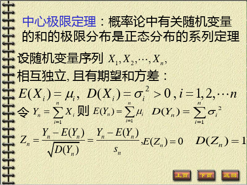
独立同一分布, 且有期望和方差:
E( X k ) , D( X k ) 2 0 , k 1,2,
则对于任意实数 x ,
n
Xk
n
lim P k1
x
n
n
1
x
e
t2
2 dt
(x)
2
n
注
X k n
记 Yn k1 n
n
则 Y n 为 X k 的标准化随机变量.
k 1
lim
n
PYn
x
( x)
即 n 足够大时,Y n 的分布函数近似于标 准正态随机变量的分布函数
近似
n Yn ~ N (0,1)
X k nYn n 近似服从N (n,n 2 )
k 1
中心极限定理的意义
在第二章曾讲过有许多随机现象服从 正态分布 是由于许多彼次没有什么相依关 系、对随机现象谁也不能起突出影响,而 均匀地起到微小作用的随机因素共同作用 (即这些因素的叠加)的结果.
测度论基础与高等概率论21章中心极限定理

测度论基础与高等概率论21章中心极限定理中心极限定理是概率论中一组重要的定理,用于研究随机变量序列的极限分布。
在测度论基础与高等概率论的21章,涉及到中心极限定理的相关内容,以下是一些相关参考内容:1. 弱大数定律:弱大数定律是中心极限定理中的一种形式,它陈述了当独立同分布(i.i.d.)的随机变量序列的方差有限时,序列的算术平均值以概率1收敛到其数学期望。
弱大数定律表明了当样本容量足够大时,随机变量序列的平均值在概率上趋近于其数学期望。
2. 中心极限定理的基本思想:中心极限定理的基本思想是指出,当独立随机变量的和在适当缩放后对于任意给定的实数都收敛到标准正态分布。
中心极限定理提供了一种将原始数据与正态分布联系起来的方法。
3. 林德伯格中心极限定理:林德伯格中心极限定理是中心极限定理的一种形式,它陈述了当随机变量来自于任何分布(不一定是独立同分布的)且具有有限的均值和方差时,它们的标准化和服从于标准正态分布。
林德伯格中心极限定理是中心极限定理的一般化,适用范围更广。
4. 切比雪夫不等式:切比雪夫不等式是中心极限定理中的一种工具,它提供了一种估计随机变量与其数学期望之间差距的方法。
切比雪夫不等式指出,对于任意正数ε,当随机变量的方差有限时,不等式P(|X-μ|≥ε)≤σ²/ε²成立,其中X是随机变量,μ是其数学期望,σ是其标准差。
5. 中心极限定理在统计推断和假设检验中的应用:中心极限定理在统计推断和假设检验中具有重要应用。
它可以用来进行参数估计、构造置信区间和进行假设检验。
基于中心极限定理,可以构造统计量,并根据标准正态分布来计算容易估算的概率。
综上所述,中心极限定理是测度论基础与高等概率论中的一个重要内容。
它提供了在独立随机变量序列的极限分布研究中的有力工具,深刻揭示了随机现象背后的规律性。
此外,中心极限定理具有广泛的应用,可以用于统计推断和假设检验等领域,为实际问题的分析和解决提供了有力的数学工具。
概率论与数理统计第4章 随机变量的数字特征与极限定理

25
定义4.3 设X是随机变量,若E[X-E(X)]2存 在,则称它为X的方差,记为D(X),即
由定义4.2,随机变量X的方差反映了X的可能取值 与其数学期望的平均偏离程度.若D(X)较小,则X的 取值比较集中,否则,X的取值比较分散.因此,方差 D(X)是刻画X取值离散程度的一个量.
3
定义4.1 设离散型随机变量X的分布律为
4
5
6
7
8
9
4.1.2 几个常用分布的数学期望 1.0—1分布 设随机变量X服从以p为参数的(0—1)分布,则X 的数学期望为
2.二项分布 设随机变量X~B(n,p),则X的数学期望为
10
3.泊松分布 设随机变量X~P(λ)分布,则X的数学期望为
41
Hale Waihona Puke 424.3 协方差、相关系数及矩
4.3.1 协方差 对于二维随机变量(X,Y),除了分量X,Y的数 字特征外,还需要找出能体现各分量之间的联系的数字 特征.
43
44
4.3.2 相关系数 定义4.5 设(X,Y)为二维随机变量,cov (X,Y),D(X),D(X)均存在,且D(X)>0,D(X) >0,称
15
16
17
定理4.2 设(X,Y)是二维随机变量,z=g(x,y) 是一个连续函数. (1)如果(X,Y)为离散型随机变量,其联合分布 律为
18
19
20
4.1.4 数学期望的性质 数学期望有如下常用性质(以下的讨论中,假设所 遇到的数学期望均存在):
随机变量序列的极限

x 为标准正态分布的分布函数.
n X i n lim P i 1 x x . n n
该定理的实际意义是, 若随机变量序列 X1 , X 2 , 满足定理条件, 记 Yn
X i , 则当n充分大时
i 1
所以原概率近似为
64 P X i 7000 0.2266. i 1
B 1, p , i 1,2,, 则 E X i p, D X i pq 0, 即随机变量序列
作为上面定理的特例, 如果 X i
满足上面定理的条件. 从而有下面的定理.
A, A,
引进随机变 量
1 Xi 0
第i次试验A发生 第i次试验A发生
Xi ~ B 1, p , E Xi p, i 1,2., n,
X1 , X 2 ,, X n
频率
p 1 f n A X i X P A p n i 1 n
由条件所设, 所求的概率为
x 0.99.
而 x 为标准正态分布的分布函数, 查表得 x 2.326. 即:
N 300 Q 2.326. 5 3 从而 3 N 300 2.326 20 Q 4
300 20 Q 320Q.
P Xn c.
若随机变量序列 X1 , X 2 , 依概率收敛于c, 则
lim P X n c 0.
n
定理
a, b 处连续,
如果 X n
a, Yn b, 且函数 g x, y 在点 P 则 g X n , Yn a, b.
相互独立,则在n次ຫໍສະໝຸດ 验中A发生的例1 设 X1 , X 2 ,是独立同分布的随机变量序列, 且
相依随机变量列的极限定理
其中 ^ 与 , 2是任 何 两个使 得协 方差 存 在 的对 每 个变量 均 非 降( 非升) 函数 。称随机 变 或 的
量序列 { i ∈ X , Ⅳ)是 N i A序列,如果对任何 n 2 ,随机变量 1 , , n≥ 2 都 , … 2 )
(5 Z 5、 0 E 3)
维普资讯
40 7
工
程
数
学
学 Hale Waihona Puke 报 第 2 卷 4
本 文首先 引入渐 近负相关随机变量序 列的定义 ,获得这种序列 的大 数律 ,并将伯恩斯坦大 数律作 为本文结果的特例而得到 。其次,证 明了定理 C等价于 L de定理 ,并讨论了一般相依 ov
是 NA 的 。
定义2。 随机 变量 和 y 是 N [ 】 QD 的 ( gt e udat p net,若对 V , Neai l Q arn edn) vy De xY∈
R,有
PX< Y<Y PX <x ( . ( , ) ( ) Y< ) P
称随机变量列 { nn 1 是两两 N D的,若对 V ≠JX 与 z , ) Q i , i 是 N D 的。 Q 定义3 称随机变量列 { , 1 n >是 A A( sm tt a N gt e s c t ) N A y po cl ea vl A s i e 的,如 i i y oad 果对 于任意给定的 E ,存在 N >0 >0 ,当 I—J> N 时 ,cvX ̄ ) 。 i I o ( , <E 定义4 1 两个随机变量序列 { 几 1 和 {nn 1 称为等价的,如果 [] 1 , ) 叩 , )
它大数律相继出 见文 『 11 现( 5 2 。这些结果都是将独立随机变量列的强弱大数律向两两 N D列 , ) Q
随机过程第01章 基础知识772.7 2.7 收敛性和极限定理
(3)若 X n 依概率收敛,则 X n 必为依分布收敛。
注 均方收敛与以概率1收敛不存在确定的关系。
二、极限定理
1.强大数定理
如果 X1,X 2, 独立同分布,
具有均值 ,则
首页
P{lim ( n
X1
X
2
X
n
)
/
n
}
1
2.中心极限定理 如果 X1,X 2, 独立同分布,
设 Fn (x),F(x)分别为随机变量 X n 及X 的
分布函数
如果 F(x) 对于的每一个连续点x,有
lim
n
Fn
(x)
F
(x)
则称 随机变量序列 X n 以分布收敛于X,记作
X n d X
首页
收敛性之间的关系
(1)若
X
均方收敛,则
n
X n 必为依概率收敛;
(2)若 X n 以概率1收敛,则 X n 必为依概率收敛;
具有均值 与方差 2 ,则
lim P X1 X n n a
n
n
a
1
x2
e 2 dx
2
n
注 若令 Sn X i ,其中 X1,X 2, 独立同分布 i 1
则 强大数定理 表明 Sn / n 以概率1收敛于 E[X i ];
中心极限定理 表明当n 时,S n 有
且
lim
n
E[|
Xn
X
|2 ]
0
则称 随机变量序列 X n 以均方收敛于X,记作
l.i.m n
Xn
X
随机变量序列极限

i 1
n
Xi
B 1, p ,
则
X
i 1
n
i
B n, p ,
进一步地有
X
则
B m, p , Y
B n, p ,
X Y
有这个必要.
B m n, p .
但很多情况下这样的分布并不能得到, 有时也不一定
人们在长期实践中发现 , 在相当一般的条件下, 只要 n
该定理的实际意义是, 若随机变量序列 X1 , X 2 , 满足定理条件, 记 Yn
X i , 则当n充分大时
i 1
n
Yn E Yn D Yn
近似服从标准正态分布. 即
Yn X i ~ N E Yn , D Yn .
i 1
n
.
例2 某人要测量甲、乙两地的距离, 限于测量工具, 他 分成1200段进行测量, 每段测量误差(单位: 厘米)服从
注意
该定理的条件为方差有界.
定理
(独立同分布情形下的大数定律) 设 X1 , X 2 ,
2
是独立同分布的随机变量序列, 且 E
D X i , i 1, 2,
,
则
X .
P
X i ,
用独立同分布情形下的大数定律可以证明频率的稳 定性。 设进行n次独立重复的试验,每次试验只有两个结果
第五章 随机变量序列的极限
本章要点
本章讨论两类重要的极限分布.
一、大数定律
定义 设 数c, 使得对于任意常数 0, 总有
n
X1 , X 2 ,
是一个随机变量序列, 如果存在常
概率论第五章大数定律与中心极限定理讲解

1 P
1200
Xk
k 1
10
0
2
1[
2
2
]
2 22 2 0.0228 0.0456
例2 根据以往经验,某种电器元件的寿命服从均 值为100小时的指数分布. 现随机地取16只,设它们的 寿命是相互独立的. 求这16只元件的寿命的总和大于 1920小时的概率.
可知,当 n 时,有 1nn 源自1XiP E( X1)
a
因此我们可取 n 次测量值 x1, x2, , xn 的算术平均值
作为a
得近似值,即
a
1 n
n i1
xi ,当n充分大时误差很小。
例4 如何估计一大批产品的次品率 p ? 由伯努利大数定律可知,当 n 很大时,可取频率
则对任意的 x ,有
n ~ N(np, np(1 p)) n , 近似地
即 n np ~ N (0,1)
np(1 p)
或 lim P{ n np
x
x}
1
t2
e 2 dt x
n np(1 p)
2
证 因为 n ~ b(n, p)
n
所以 n X k k 1
i 1
1200
1200
心极限定理可得 X k ~ N (n,n 2),即 X k ~ N (0,100)
k 1
k 1
则所求概率为
1200
1200
P k1 X k
20
P
Xk 0
k 1
第八章独立随机变量和的极限定理

第八章 独立随机变量和的极限定理8.1 0-1律设(为概率空间,事件序列)P ,,F ΩF ∈L ,,21A A ,表示事件有无穷多个发生(happens infinitely often),记为IU ∞=∞=1n n k k A n A {}..o i A n ni A ,即;表示至多有限个不发生(happens for all but finitely many ),注意;若用示性函数表示{}, {}n o i A ..= =∑∞:.n w n n nk k A A 1∞=∞==IU n =1)(.A w I o n n _____lim ∞→∞=UI ∞=∞=1n n k An nk A ∞=∞=1UI kn A n n k A ∞→=____lim ∞<)(A w I n ∑∞=1:n kw =∞=∞=1n nk A UI 。
定理1:(Borel-Cantelli Lemma)若,则∞<∑∞=1)(n n A P ()0..=o i A P n ;若独立且,则。
{n A }}}∞=∑∞=1)(n nA P ()1..=o i A P n推论1:(Borel 0-1 law)设{为独立事件序列,则n A ()∞=∞<=∑∑∞=∞=.)(,1,)(,0..11n n n n n A P A P o i A P 当当 推论2:设{n ξ为独立随机变量序列,则()∞<≥>∀⇔ → ∑∞=1..,00n n s a n c P c ξξ。
证明:令{c A n n ≥=ξ}},由推论1立得。
定义1:设{}{n n ηξ,为两个随机变量序列,若()0..=≠o i P n n ηξ,则称{}{}n n ηξ,尾等价。
注意尾等价的含义:(0..)=≠o i n n P ηξ表明使得{}{})(,)(w w n n ηξ中有无穷多项不等的w 是一个零测集,设为M ,这意味着在M w ∈上,{}{})(w n ,)(w n ηξ只是有限个不等,故对每一M )(w N w ∈,存在,当时)(w N >n )()(w w n n ηξ=。
Ch5.2 中心极限定理

例3 对于一个学生而言,来参加家长会的家长人数 对于一个学生而言,
是一个随机变量, 个学生无家长、 1名家长、 2名 是一个随机变量,设一 个学生无家长、 名家长、 家长来参加会议的概率 分别为 .05 0.8、15.若学校 0 、 0. 共有400名学生,设各学生参加 名学生, 会议的家长数相互 独立, 独立,且服从同一分布.
概率论与数理统计
第二节
中心极限定理
中心极限定理 例题 课堂练习
中心极限定理的客观背景 在实际问题中许多随机变量是由相互独立随机 因素的综合(或和)影响所形成的 影响所形成的. 因素的综合(或和 影响所形成的 例如: 例如:炮弹射击的 落点与目标的偏差, 落点与目标的偏差, 就受着许多随机因 如瞄准, 素(如瞄准,空气 阻力,炮弹或炮身结构等)综合影响的.每个随机因 阻力,炮弹或炮身结构等)综合影响的 每个随机因 素的对弹着点(随机变量和)所起的作用都是很小 素的对弹着点(随机变量和) 的.那么弹着点服从怎样分布哪 ? 那么弹着点服从怎样分布哪
相互独立, 设随机变量X1, X2 ,LXn ,L相互独立,服从同一分 方差: E( Xk ) = µ, D( Xk ) = σ 2 布,且具有数学期望和 (k = 1,2,L,则随机变量之和 ∑ Xk的标准化变量 )
n
Yn = k=1
∑ Xk − nµ n σ
n
k=1
F x 的分布函数 n( x)对于任意 满足
设需N台车床工作, 现在的问题是: 设需 台车床工作, 现在的问题是: 台车床工作 求满足 P(X≤N)≥0.999 的最小的N. 的最小的
千瓦, 台工作所 (由于每台车床在开工时需电力1千瓦,N台工作所 由于每台车床在开工时需电力 千瓦 需电力即N千瓦 千瓦.) 需电力即 千瓦 )
- 1、下载文档前请自行甄别文档内容的完整性,平台不提供额外的编辑、内容补充、找答案等附加服务。
- 2、"仅部分预览"的文档,不可在线预览部分如存在完整性等问题,可反馈申请退款(可完整预览的文档不适用该条件!)。
- 3、如文档侵犯您的权益,请联系客服反馈,我们会尽快为您处理(人工客服工作时间:9:00-18:30)。
n i 1
Xi
1 n
n i 1
E
Xi
P 0.
特别地, 若E Xi ,i 1, 2, , 则上式表明
X
1 n
n i 1
Xi
P
.
注意 该定理的条件为方差有界.
定理 (独立同分布情形下的大数定律) 设 X1, X 2 ,
是独立同分布的随机变量序列, 且E Xi , D Xi 2,i 1, 2, , 则 X P .
得
E
X
i
0,
D
X
i
1 12
,
i 1,2, ,1200.
E
1200 i1
X
i
1200
0
0,
D
1200 i1
X
i
1200
1 12
=100
由独立同分布的中心极限定理:
n
.
Xi ~ N 0,100
i 1
1200
P Xi
20
1
P
20
1200
X
i
20
i1
i 1Βιβλιοθήκη 120 100
20 10
0
1 2 2
21 2 0.0456.
作为上面定理的特例, 如果 Xi B1, p,i 1, 2, , 则 E Xi p, D Xi pq 0, 即随机变量序列
满足上面定理的条件. 从而有下面的定理.
定理 (中心极限定理 )设 X1, X 2 , 是一个独立同分
时很困难. 有些情况下, 可以得到其分布. 例如
Xi B1, p, 则
n
Xi B n, p,
i 1
进一步地有
X Bm, p,Y Bn, p,
则
X Y Bm n, p.
但很多情况下这样的分布并不能得到, 有时也不一定
有这个必要.
人们在长期实践中n 发现, 在相当一般的条件下, 只要
n充分大, 总认为 Xi 近似服从正态分布. i1 下面这个例子说明了这个情况.
例 (高尔顿钉板实验) 高尔顿设计了一个钉板实验, 图中每个黑点表示钉在板上的一个钉子, 它们彼此间的 距离相等, 上一层的每一个钉子的水平位置恰好位于下 一层的两个钉子的正中间. 从入口处放进一个直径略小 于两个钉子之间的距离的小球. 在小 球向下降落的过程中, 碰到钉子后均
以0.5的概率向左或向右滚下, 于是
分成1200段进行测量, 每段测量误差(单位: 厘米)服从
区间0.5,0.5上的均匀分布, 试求总距离测量误差的
绝对值超过 20 厘米的概率.
1200
解 设第i 段的测量误差为 X i , 所以累计误差为 X i , i 1
又 X1, X 2 , , X1200 为独立同分布的随机变量, 由
Xi R0.5,0.5
Xk
1,
1,
小球碰第 k层钉后向右落下 小球碰第 k层钉后向左落下
(k 1, 2,,16)
程序如下
输出图形
定理 (独立同分布的中心极限定理)设 X1, X 2 , 是
独立同分布的随机变量序列, 且
E Xi ,D Xi 2 0 则对任意的 x x , 有
i 1,2, ,
n
Xi n
fn
A
1 n
n i 1
Xi
X
p
P A
p
例1 设 X1, X 2 , 是独立同分布的随机变量序列, 且
E Xi , D Xi 2,i 1, 2, , 则
1
n
n i 1
X
2 i
P 2
2.
二、中心极限定理
在数理统计中经常要用到 n个独立同分布的随机变量
n
X1, X 2, , X n的和 X i 的分布, 但要给出其精确分布有 i 1
又碰到下一层钉子. 如此进行下去, 直 到滚到底板的一个格子里为止. 把许
多同样大小的小球不断从入口处放下, 只要球的数目相
当大, 它们在底板将堆成近似正态分布 N 0, 2 的密
度函数图形.
高尔顿( Francis Galton,18221911) 英国人类 学家和气象学家
共16层小钉
x -8 -7 -6 -5 -4 -3 -2 -1 O1 2 3 4 5 6 7 8
解 令X 表示在时刻 t 时正在开动的机器数, 则
X B400,0.75.
优选Ch随机变量序列的极限
本章要点
本章讨论两类重要的极限分布.
一、大数定律
定义 设 X1, X 2 , 是一个随机变量序列, 如果存在常
数c, 使得对于任意常数 0, 总有
lim P
n
Xn c
1,
则称随机变量序列 X1, X 2 , 依概率收敛于c, 记作
X n P c.
若随机变量序列 X1, X 2 , 依概率收敛于c, 则
lim P
n
Xn c
0.
定理 如果 X n P a,Yn P b, 且函数 g x, y 在点
a,b 处连续, 则 g Xn,Yn P a,b.
定理 设 X1, X 2 , 是两两不相关的随机变量序列, 如
果存在常数 c, 使得 D Xi c,i 1, 2, , 则
1
lim P i1
x x.
n
n
其中 x 为标准正态分布的分布函数.
该定理的实际意义是,
若随机变量序列
n
X1,
X
2
,
满足定理条件, 记 Yn X i , 则
i 1
Yn E Yn
D Yn
近似服从标准正态分布.
n
.
即 Yn Xi ~ N E Yn , D Yn .
i 1
例2 某人要测量甲、乙两地的距离, 限于测量工具, 他
用独立同分布情形下的大数定律可以证明频率的稳 定性。
设进行n次独立重复的试验,每次试验只有两个结果
A, A, 引进随机变
量
1 第i次试验A发生
Xi 0 第i次试验A发生
Xi ~ B1, p, E Xi p,i 1,2. ,n,
X1, X 2 , , X n 相互独立,则在n次试验中A发生的
频率
X np
np1 p
.
近似服从标准正态分布.即 X ~ N np,np1 p .
例3 设一个车间有400台同类型的机床, 每台机床需用
电 Q瓦, 由于工艺关系, 每台机器并不连续开动, 开动的 时候只占工作总时间的3/ 4, 问应该供应多少瓦电力能
99%的概率保证该车间的车床能正常工作.(假定在工作 期内每台机器是否处于工作状态是相互独立的).
布的随机变量序列, 且 Xi B1, p, 令
n
Yn Xi , i 1
则对任意的 x x , 有
lim P
Yn np
x
1
x t2
e 2 dt,
n np 1 p 2π
即当 n充分大时, Yn np 近似服从标准正态分布. np1 p
该定理的实际意义是: 若 X Bn, p, 则