滚子摆动从动件凸轮设计matlab程序
基于MATLAB的凸轮轮廓线设计与运动仿真毕业设计
(此文档为word格式,下载后您可任意编辑修改!)第1章绪论1.1 机构学的现状与发展1.1.1 机构学的概况机构学是以运动几何学和力学为主要理论基础,以数学分析为主要手段,对各类机构进行运动和动力分析与综合的学科。
机构学为创造新的机器和进行机械发明与改革提供正确有效的理论和方法,以设计出更经济合理、更先进的机械设备,来满足生产发展和人们生活的需求。
机构学的发展将直接影响到机械工业各类产品的工作性能以及许多行业生产设备的机械化和自动化程度。
机构学作为机械工程技术科学中的一门主要基础学科,近年来由于机电一体化高技术科学特别是工业机器人与特种机器人的发展对机构学理论和技术上的要求,使机构学学科达到了一个崭新的阶段。
在国际学术讨论会上,各国科学家一致认为它有如旭日东升,正显出其无比强大的生命力。
机构学一方面由简单的运动分析与综合向复杂的运动分析与综合方面发展,另一方面也由机构运动学向机构动力分析与综合方向发展,研究机构系统的合理组成的方法及其判据,分析研究机器在传递运动、力和做功过程中出现的各种问题。
机构精度问题也相应地由静态分析走向动态分析。
机构联结件的间隙在高速运转时有不容忽视的影响,因而需要研究机构间间隙、摩擦、润滑与冲击引起的机构变形、稳态与非稳态下的动态响应和过渡过程问题。
在惯性力作用下,由于机构上刚度薄弱环节的弹性变形,由此研究以振动理论多自由度模态化、线性与非线性、随机的功率谱与载荷谱等为分析手段和方法而形成的运动弹性动力学问题,以及视整个机构系统为柔性的多柔体系统动力学和逆动力学分析、综合及控制问题。
它是把整个机构看成是由多刚体组成的多刚体动力学、结构动力学及自动控制等学科发展的交叉边缘学科。
由多种、多个构件组成的机构称为组合机构。
组合机构与机构系统组成理论的发展使机构学已成为重型、精密及各种复合机械和智能机械、仿生机械、机器人等高技术科学的设计基础理论学科。
1.1.2机构学的现状(1)平面与空间连杆机构的结构理论研究研究机构的结构单元及机构拓扑结构特征,如主动副存在准则、活动度类型及其判定、拓扑结构的同构判定、消极子运动链判定等。
基于MATLAB的凸轮设计
基于MATLAB的凸轮设计凸轮是一种用于转动机件的机械元件,常用于驱动一些运动部件做往复运动或者周期性运动。
在机械设计中,通过凸轮的设计可以实现复杂的运动路径,以及具有特定速度和加速度要求的运动。
MATLAB是一种强大的数学计算和编程环境,可以用于进行科学计算、数据分析和算法开发。
在凸轮设计中,MATLAB可以用于凸轮曲线的生成、设计和优化。
本文将介绍如何基于MATLAB进行凸轮设计。
在凸轮设计中,最重要的是凸轮曲线的生成。
凸轮曲线是一个由数据点组成的模板,通过插值或者数值逼近的方法可以生成一个光滑的凸轮曲线。
在 MATLAB 中,可以使用插值函数 interp1 或者曲线拟合函数polyfit 进行凸轮曲线的生成。
具体步骤如下:1.定义凸轮的设计参数,例如凸轮的半径、凸轮转动的角度范围等;2.根据凸轮的设计参数,生成一些数据点,这些数据点可以通过数学计算或者几何建模等方式得到;3. 使用插值函数 interp1 或者曲线拟合函数 polyfit 对这些数据点进行插值或者拟合,得到一个平滑的曲线;4.根据凸轮转动的角度范围,生成一系列角度的数据点;5. 使用插值函数 interp1 或者曲线拟合函数 polyval 对这些角度的数据点进行插值或者拟合,得到一系列对应的曲线坐标点;6.将这些坐标点绘制成凸轮曲线,并进行可视化。
除了凸轮曲线的生成,MATLAB 还可以用于凸轮的设计和优化。
凸轮设计包括凸轮的尺寸设计、运动路径设计等。
在 MATLAB 中,可以使用优化函数 fmincon 或者遗传算法函数 ga 进行凸轮设计的优化,以获得符合设计要求的凸轮参数。
具体步骤如下:1.定义凸轮的设计变量和目标函数。
设计变量可以是凸轮的尺寸参数,例如凸轮半径、凸轮高度等;目标函数可以是凸轮的运动路径误差、速度误差等。
2.定义凸轮的约束条件。
约束条件可以是凸轮的尺寸范围、速度和加速度的限制等。
3. 使用优化函数 fmincon 或者遗传算法函数 ga 对凸轮的设计变量进行优化,以使目标函数最小化或者最大化。
基于MATLAB的摆动式磨头圆柱端面凸轮曲线优化设计
4 0 40
2 l5 r l 2 。 7 ( 耵 一7 7 ( , 一7 一7 ) 2 25 r 1—7 ) 2
() 5
2 3 约束 条件 . 2 3 1 转 角 . .
要求 , 取
1
和 : 的要求
为保证 摆杆 在 中段匀 速 摆 动 , 足 磨 头磨 削工 艺 满
图 1 凸轮 机构 压 力角
Fiu e 1 Ca me h nim r su e a ge g r m c a s p e s r n l
1+ 2≤ 订
() 6
2 34 主 动摆杆 与 凸轮干 涉 .. 将 圆柱 凸轮展 开成平 面便 成 为移 动 凸轮 ¨ 建 立 , 凸轮转 角为横 坐标 , 曲线 高 度 为纵 坐 标 的 平 面直 角 坐
模型 , 用 MA L B软件的功能 函数 cnt求得优化结果。优化后最大无 因次加速度为优 化前的 3 % , 运 TA os r 3 和原有 曲线相 比
下降了3 %, 0 可以有效的降低磨头的振动及故障率, 提高陶瓷地砖加工的表面质量, 降低震碎率。图7参 1 1
关 键 词 : 瓷抛 光 机 ; 化 设 计 ; T A 软 件 ; 柱 端 面 凸轮 陶 优 MA L B 圆
Ab t a t T mp o e d n mi c p b l y o r d n e d c m c a i o e a c p l h n c i e a i g t e sr c : o i r v y a c a a i t f g n i g h a a me h ns i i m f c r mi o i i g ma h n , t k n h s
滚子摆动从动件凸轮设计matlab程序
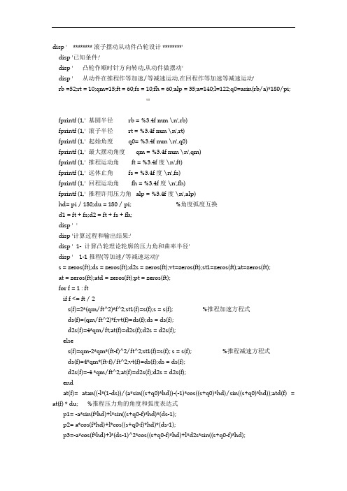
disp ' ******** 滚子摆动从动件凸轮设计 ********'disp '已知条件:'disp ' 凸轮作顺时针方向转动,从动件做摆动'disp ' 从动件在推程作等加速/等减速运动,在回程作等加速等减速运动'rb =52;rt = 10;qm=15;ft = 60;fs = 10;fh = 60;alp = 35;a=140;l=122;q0=asin(rb/a)*180/pi;fprintf (1,' 基圆半径 rb = %3.4f mm \n',rb)fprintf (1,' 滚子半径 rt = %3.4f mm \n',rt)fprintf (1,' 起始角度 q0= %3.4f mm \n',q0)fprintf (1,' 最大摆动角度 qm = %3.4f mm \n',qm)fprintf (1,' 推程运动角 ft = %3.4f 度 \n',ft)fprintf (1,' 远休止角 fs = %3.4f 度 \n',fs)fprintf (1,' 回程运动角 fh = %3.4f 度 \n',fh)fprintf (1,' 推程许用压力角 alp = %3.4f 度 \n',alp)hd= pi / 180;du = 180 / pi; %角度弧度互换d1 = ft + fs;d2 = ft + fs + fh;disp ' 'disp '计算过程和输出结果:'disp ' 1- 计算凸轮理论轮廓的压力角和曲率半径'disp ' 1-1 推程(等加速/等减速运动)'s = zeros(ft);ds = zeros(ft);d2s = zeros(ft);vt=zeros(ft);st1=zeros(ft);at=zeros(ft);at = zeros(ft);atd = zeros(ft);pt = zeros(ft);for f = 1 : ftif f <= ft / 2s(f)=2*(qm/ft^2)*f^2;st1(f)=s(f);s = s(f); %推程加速方程式ds(f)=(qm/ft^2)*f;vt(f)=ds(f);ds = ds(f);d2s(f)=4*qm/ft;at(f)=d2s(f);d2s = d2s(f);elses(f)=qm-2*qm*(ft-f)^2/ft^2;st1(f)=s(f); s = s(f); %推程减速方程式ds(f)=4*qm*(ft-f)/ft^2;vt(f)=ds(f);ds = ds(f);d2s(f)=-4 *qm/ft^2;at(f)=d2s(f);d2s = d2s(f);endat(f)= atan((-l*(1-ds))/(a*sin((s+q0)*hd))-(-1)*cos((s+q0)*hd)/sin((s+q0)*hd));atd(f) = at(f) * du; %推程压力角的角度和弧度表达式p1= -a*sin(f*hd)+l*sin((s+q0-f)*hd)*(ds-1);p2= a*cos(f*hd)+l*cos((s+q0-f)*hd)*(ds-1);p3=-a*cos(f*hd)+l*(ds-1)^2*cos((s+q0-f)*hd)+l*d2s*sin((s+q0-f)*hd);p4=-a*sin(f*hd)-l*(ds-1)^2*sin((s+q0-f)*hd)+l*ds*cos((s+q0-f)*hd);pt(f)= (p1^2+p2^2)^1.5/(p1*p4-p2*p3) ;p = pt(f);endatm = 0;for f = 1 : ftif atd(f) > atmatm = atd(f);endendfprintf (1,' 最大压力角 atm = %3.4f 度\n',atm)for f = 1 : ftif abs(atd(f) - atm) < 0.1ftm = f;breakendendfprintf (1,' 对应的位置角 ftm = %3.4f 度\n',ftm)if atm > alpfprintf (1,' * 凸轮推程压力角超过许用值,需要增大基圆!\n')endptn = rb ;ftn=0;for f = 1 : ftif pt(f) < ptnptn = pt(f);endendfprintf (1,' 轮廓最小曲率半径 ptn = %3.4f mm\n',ptn)for f = 1 : ftif abs(pt(f) - ptn) < 0.1ftn = f;breakendendfprintf (1,' 对应的位置角 ftn = %3.4f 度\n',ftn)if ptn < rt + 5fprintf (1,' * 凸轮推程轮廓曲率半径小于许用值,需要增大基圆或减小滚子!\n') enddisp ' 1-2 回程(等加速等减速运动)'s = zeros(fh);ds = zeros(fh);d2s = zeros(fh);ah = zeros(fh);ahd = zeros(fh);ph = zeros(fh);for f = d1 : d2k = f - d1;if k<=fh / 2s(f) =qm-2*qm*(k)^2/fh^2;st1(f)=s(f); s = s(f);ds(f)=-4*qm*k/fh^2;ds = ds(f);d2s(f)= -4*qm/fh^2;d2s = d2s(f);elses(f) =2*qm*(d2-f)^2/fh^2;st1(f)=s(f); s = s(f);ds(f)=-4*qm*(d2-f)/fh^2;ds = ds(f);d2s(f)=4*qm/fh^2;d2s = d2s(f);endat(f)= atan((-l*(1-ds))/(a*sin((s+q0)*hd))-(-1)*cos((s+q0)*hd)/sin((s+q0)*hd));atd(f) = at(f) * du; %推程压力角的角度和弧度表达式p1= -a*sin(f*hd)+l*sin((s+q0-f)*hd)*(ds-1);p2= a*cos(f*hd)+l*cos((s+q0-f)*hd)*(ds-1);p3=-a*cos(f*hd)+l*(ds-1)^2*cos((s+q0-f)*hd)+l*d2s*sin((s+q0-f)*hd);p4=-a*sin(f*hd)-l*(ds-1)^2*sin((s+q0-f)*hd)+l*ds*cos((s+q0-f)*hd);pt(f)= (p1^2+p2^2)^1.5/(p1*p4-p2*p3) ;p = pt(f);endatm = 0;for f = 1 : ftif atd(f) > atmatm = atd(f);endendfprintf (1,' 最大压力角 atm = %3.4f 度\n',atm)for f = 1 : ftif abs(atd(f) - atm) < 0.1ftm = f;breakendendfprintf (1,' 对应的位置角 ftm = %3.4f 度\n',ftm)if atm > alpfprintf (1,' * 凸轮推程压力角超过许用值,需要增大基圆!\n')endptn = rb ;ftn=0;for f = 1 : ftif pt(f) < ptnptn = pt(f);endendfprintf (1,' 轮廓最小曲率半径 ptn = %3.4f mm\n',ptn)for f = 1 : ftif abs(pt(f) - ptn) < 0.1ftn = f;breakendendfprintf (1,' 对应的位置角 ftn = %3.4f 度\n',ftn)if ptn < rt + 5fprintf (1,' * 凸轮推程轮廓曲率半径小于许用值,需要增大基圆或减小滚子!\n') enddisp ' 2- 计算凸轮理论廓线与实际廓线的直角坐标'n = 360;s = zeros(n);ds = zeros(n);r = zeros(n);rp = zeros(n);x = zeros(n);y = zeros(n);dx = zeros(n);dy = zeros(n);xx = zeros(n);yy = zeros(n);xp = zeros(n);yp = zeros(n);xxp = zeros(n);yyp = zeros(n);for f = 1 : nif f <= ft/2s(f)=2*(qm/ft^2)*f^2;s = s(f);ds(f)=(qm/ft^2)*f;ds = ds(f);elseif f > ft/2 & f <= fts(f)=qm-2*qm*(ft-f)^2/ft^2; s = s(f);ds(f)=4*qm*(ft-f)/ft^2;ds = ds(f);elseif f > ft & f <= d1s = qm;ds = 0;elseif f > d1 & f <= (d2-fh/2)k = f - d1;s(f) =qm-2*qm*(k)^2/fh^2; s = s(f);ds(f)=-4*qm*k/fh^2;ds = ds(f);elseif f>(d2-fh/2)&f<=d2s(f) =2*qm*(d2-f)^2/fh^2; s = s(f);ds(f)=-4*qm*(d2-f)/fh^2;ds = ds(f);elseif f > d2 & f <= ns = 0;ds = 0;endxx(f) = a*cos(f*hd)-l*cos((s+q0-f)*hd);x=xx(f);yy(f) = a*sin(f*hd)+l*sin((s+q0-f)*hd);y=yy(f);dx(f) = -a*sin(f*hd)+l*sin((s+q0-f)*hd)*(ds-1); dx = dx(f);dy(f) = a*cos(f*hd)+l*cos((s+q0-f)*hd)*(ds-1); dy = dy(f);xp(f) = x-rt*(dy/sqrt(dx^2+dy^2));xxp=xp(f);yp(f) = y+rt*(dx/sqrt(dx^2+dy^2));yyp = yp(f);r(f) = sqrt (x ^2 + y ^2 );rp(f) = sqrt (xxp ^2 + yyp ^2 );enddisp ' 2-1 推程(等加速/等减速运动)'disp ' 凸轮转角理论x 理论y 实际x 实际y'for f = 10 : 10 :ftnu = [f xx(f) yy(f) xp(f) yp(f)];disp(nu)enddisp ' 2-2 回程(等加速/等减速运动)'disp ' 凸轮转角理论x 理论y 实际x 实际y'for f = d1 : 10 : d2nu = [f xx(f) yy(f) xp(f) yp(f)];disp(nu)enddisp ' 2-3 凸轮轮廓向径'disp ' 凸轮转角理论r 实际r'for f = 10 : 10 : nnu = [f r(f) rp(f)];disp(nu)enddisp '绘制凸轮的理论轮廓和实际轮廓:'plot(xx,yy,'r-.') % 理论轮廓(红色,点划线)axis ([-(150) (150) -(150) (150)]) % 横轴和纵轴的下限和上限 axis equal % 横轴和纵轴的尺度比例相同text(50,0,'X') % 标注横轴text(0,50,'Y') % 标注纵轴text(-5,5,'O') % 标注直角坐标系原点title('摆动从动件盘形凸轮设计') % 标注图形标题 hold on; % 保持图形plot([-(rb) (rb)],[0 0],'k') % 横轴(黑色)plot([0 0],[-(rb) (rb+rt)],'k') % 纵轴(黑色)ct = linspace(0,2*pi); % 画圆的极角变化范围 plot(rb*cos(ct),rb*sin(ct),'g') % 基圆(绿色)plot(xp,yp,'b') % 实际轮廓(蓝色)。
凸轮廓线设计MATLAB程序
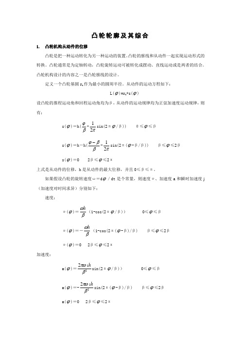
凸轮轮廓及其综合1. 凸轮机构从动件的位移凸轮是把一种运动转化为另一种运动的装置。
凸轮的廓线和从动件一起实现运动形式的转换。
凸轮通常是为定轴转动,凸轮旋转运动可被转化成摆动、直线运动或是两者的结合。
凸轮机构设计的内容之一是凸轮廓线的设计。
定义一个凸轮基圆r b 作为最小的圆周半径。
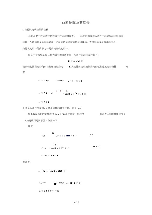
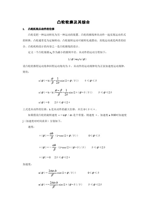
从动件的运动方程如下:L(ϕ)=r b +s(ϕ)设凸轮的推程运动角和回程运动角均为β,从动件的运动规律均为正弦加速度运动规律,则有:s(ϕ)=h(βϕ-π21sin(2πϕ/β)) 0≤ϕ≤β s(ϕ)=h -h(ββϕ--π21sin(2π(ϕ-β/β)) β≤ϕ≤2β s(ϕ)=0 2β≤ϕ≤2π上式是从动件的位移,h 是从动件的最大位移,并且0≤β≤π。
如果假设凸轮的旋转速度ω=d ϕ/dt 是个常量,则速度υ、加速度a 和瞬时加速度j (加速度对时间求异)分别如下:速度:υ(ϕ)=βωh (1-cos(2πϕ/β)) 0≤ϕ≤β υ(ϕ)=-βωh (1-cos(2π(ϕ-β)/β) β≤ϕ≤2β υ(ϕ)=0 2β≤ϕ≤2π加速度:a(ϕ)=222βπωhsin(2πϕ/β)) 0≤ϕ≤βa(ϕ)=-222βπωhsin(2π(ϕ-β)/β) β≤ϕ≤2βa(ϕ)=0 2β≤ϕ≤2π瞬时加速度:j(ϕ)=3324βωπhcos(2πϕ/β)) 0≤ϕ≤βj(ϕ)=-3324βωπhcos(2π(ϕ-β)/β) β≤ϕ≤2βj(ϕ)=0 2β≤ϕ≤2π定义无量纲位移S=s/h 、无量纲速度V=υ/ωh 、无量纲加速度A=a/h ω3和无量纲瞬时加速度J=j/h ω3。
若β=60°,则如下程序可以对以上各个量进行计算。
beta=60*pi/180;phi=linspace(0,beta,40);phi2=[beta+phi];ph=[phi phi2]*180/pi;arg=2*pi*phi/beta;arg2=2*pi*(phi2-beta)/beta;s=[phi/beta-sin(arg)/2/pi 1-(arg2-sin(arg2))/2/pi];v=[(1-cos(arg))/beta-(1-cos(arg2))/beta];a=[2*pi/beta^2*sin(arg)2*pi/beta^2*sin(arg2)];j=[4*pi^2/beta^3*cos(arg)4*pi^2/beta^3*cos(arg2)]:subplot(2,2,1)plot(ph,s,ˊK ˊ)xlabel(ˊCam angle(degrees)ˊ)ylabel(ˊDisplacement(S)ˊ)g=axis; g(2)=120; axis(g)subplot(2,2,2)plot(ph,v,ˊk ˊ,[0 120],[0 0],ˊk--ˊ)xlabel(ˊCam angle(degrees)ˊ)ylabel(ˊVelocity(V)ˊ)g=axis; g(2)=120; axis(g)subplot(2,2,3)plot(ph,a,ˊk ˊ,[0 120],[0 0],ˊk--ˊ)xlabel(ˊCam angle(degrees)ˊ)ylabel(ˊAcceleration(A)ˊ)g=axis;g(2)=120;axis(g)subplot(2,2,4)plot(ph,j,ˊkˊ,[0 120],[0 0],ˊk--ˊ)xlabel(ˊCam angle(degrees)ˊ)ylabel(ˊJerk(J)ˊ)g=axis;g(2)=120;axis(g)2 平底盘形从动作参考下图得到如下关系:在(x,y)坐标系中,凸轮轮廓的坐标为Rx和Ry,刀具的坐标为Cx和Cy:Rx=Rcos( θ+ϕ) Ry=Rsin( θ+ϕ)C x=Ccos( γ+ϕ) C y=Ccos( γ+ϕ)其中, R=θcos L θ=arctan ⎪⎪⎭⎫ ⎝⎛ϕd dL L 1 c=γγcos c L + γ=arctan ⎪⎪⎭⎫ ⎝⎛+c L d dL γϕ/ r c 是刀具的半径,且dL/d ϕ=V(ϕ)/ω。
matlab凸轮轮廓设计及仿真说明书
滚子半径
=40
1
第一章:工作意义
1.1本次课程设计意义1.2已知条件
第二章:工作设计过程5
2.1:设计思路5
2.2:滚子从动件各个阶段相关方程6
2.பைடு நூலகம்:盘型凸轮理论与实际轮廓方程7
工工“..A作……'A程过A程
3.1:滚子从动件各各阶段MATLAB程序编制…*8
3.2:凸轮的理论实际运动仿真程序编制
12
第四章…?: •……
运行结果
17
4.1:滚子运动的位移图17
4.2:滚子运动的速度图17
4.3:滚子运动的加速度图,局部加速度图……18—
44滚子运动的仿真图19
4.5:滚子运动的理论与实际轮廓图20
6.1:参考文献
22
第一章:工作意义
1.1 本次课程设计意义凸轮是一个具有曲线轮廓或凹槽的构件, 一般为主动件, 作等速回转运动或往复直线运动。与凸轮轮廓接触,并传递 动力和实 现预定的运动规律的构件, 一般做往复直线运动或 摆动,称为从动件。凸轮机构在应用中的基本特点在于能使
程和回程。凸轮轮廓曲线决定于位移曲线的
形状。在某些机械中,位移曲线由工艺过程决定,但一般
情况下只有行程和对应的凸轮转角根据工作需要决定,而
曲线的形状则由设计者选定,可以有多种运动规律。传统的凸轮运动
规律有等速、等加速-等减速、余弦加速度和正弦 加速度等。等速运 动规律因有速度突变,会产生强烈的刚性 冲击,只适用于低速。等加 速-等减速和余弦加速度也有加速度突变,会引起柔性冲击,只适用
思路口。因此,基于MATLAB件进行凸轮机构的解析法设计,可以解
决设计工作量大的问题。
本此课程设计基于MATLAB软件进行凸轮轮廓曲线的 解析法 设计,并 对的运动规律凸轮进行仿真,其具体方法为首先精确地 计算出轮 廓线
基于MATLAB的摆动式磨头圆柱端面凸轮曲线优化设计

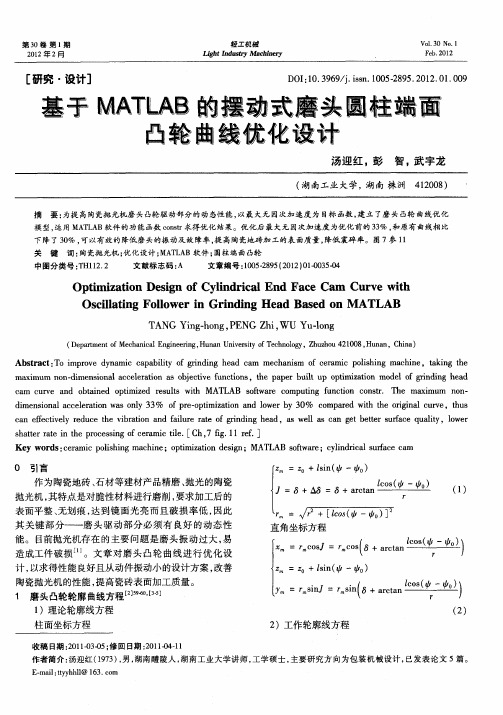
基于MATLAB的摆动式磨头圆柱端面凸轮曲线优化设计汤迎红;彭智;武宇龙【摘要】为提高陶瓷抛光机磨头凸轮驱动部分的动态性能,以最大无因次加速度为目标函数,建立了磨头凸轮曲线优化模型,运用MATLAB软件的功能函数constr求得优化结果.优化后最大无因次加速度为优化前的33%,和原有曲线相比下降了30%,可以有效的降低磨头的振动及故障率,提高陶瓷地砖加工的表面质量,降低震碎率.%To improve dynamic capability of grinding head cam mechanism of ceramic polishing machine, taking the maximum non-dimensional acceleration as objective functions, the paper built up optimization model of grinding head cam curve and obtained optimized results with MATLAB software computing function constr. The maximum non dimensional acceleration was only 33% of pre-optimization and lower by 30% compared with the original curve, thus can effectively reduce the vibration and failure rate of grinding head, as well as can get better surface quality, lower shatter rate in the processing of ceramic tile.【期刊名称】《轻工机械》【年(卷),期】2012(030)001【总页数】4页(P35-38)【关键词】陶瓷抛光机;优化设计;MATLAB软件;圆柱端面凸轮【作者】汤迎红;彭智;武宇龙【作者单位】湖南工业大学,湖南株洲412008;湖南工业大学,湖南株洲412008;湖南工业大学,湖南株洲412008【正文语种】中文【中图分类】TH112.20 引言作为陶瓷地砖、石材等建材产品精磨、抛光的陶瓷抛光机,其特点是对脆性材料进行磨削,要求加工后的表面平整、无划痕,达到镜面光亮而且破损率低,因此其关键部分——磨头驱动部分必须有良好的动态性能。
凸轮机构matlab程序
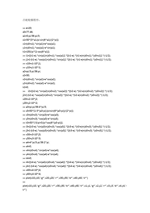
凸轮轮廓程序:>> e=20;s0=77.46;a1=0:pi/36:pi/3;s1=50*[3*a1/pi-sin(6*a1)/(2*pi)];x1=(s0+s1).*sin(a1)+e*cos(a1);y1=(s0+s1).*cos(a1)-e*sin(a1);k1=150/pi*[1-cos(6*a1)];>> i1=[(k1-e).*sin(a1)+(s0+s1).*cos(a1)].*[(k1-e).*(k1-e)+(s0+s1).*(s0+s1)].^(-1/2);>> j1=[-(k1-e).*cos(a1)+(s0+s1).*sin(a1)].*[(k1-e).*(k1-e)+(s0+s1).*(s0+s1)].^(-1/2);>> x10=x1-10*j1;>> y10=y1-10*i1;a2=pi/3:pi/36:pi;s2=50;x2=(s0+s2).*sin(a2)+e*cos(a2);y2=(s0+s2).*cos(a2)-e*sin(a2);k2=0;>> i2=[(k2-e).*sin(a2)+(s0+s2).*cos(a2)].*[(k2-e).*(k2-e)+(s0+s2).*(s0+s2)].^(-1/2);j2=[-(k2-e).*cos(a2)+(s0+s2).*sin(a2)].*[(k2-e).*(k2-e)+(s0+s2).*(s0+s2)].^(-1/2);x20=x2-10*j2;y20=y2-10*i2;>> a3=pi:pi/36:4*pi/3;>> s3=50*[1-3*(a3-pi)/pi+sin(6*(a3-pi))/(2*pi)];>> x3=(s0+s3).*sin(a3)+e*cos(a3);>> y3=(s0+s3).*cos(a3)-e*sin(a3);>> k3=50*[-3/pi+3/pi*cos(6*(a3-pi))];>> i3=[(k3-e).*sin(a3)+(s0+s3).*cos(a3)].*[(k3-e).*(k3-e)+(s0+s3).*(s0+s3)].^(-1/2);>> j3=[-(k3-e).*cos(a3)+(s0+s3).*sin(a3)].*[(k3-e).*(k3-e)+(s0+s3).*(s0+s3)].^(-1/2);>> x30=x3-10*j3;>> y30=y3-10*i3;>> a4=4*pi/3:pi/36:2*pi;>> s4=0;>> x4=(s0+s4).*sin(a4)+e*cos(a4);>> y4=(s0+s4).*cos(a4)-e*sin(a4);>> k4=0;>> i4=[(k4-e).*sin(a4)+(s0+s4).*cos(a4)].*[(k4-e).*(k4-e)+(s0+s4).*(s0+s4)].^(-1/2);>> j4=[-(k4-e).*cos(a4)+(s0+s4).*sin(a4)].*[(k4-e).*(k4-e)+(s0+s4).*(s0+s4)].^(-1/2);>> x40=x4-10*j4;>> y40=y4-10*i4;>> plot(x10,y10,'-g*',x20,y20,'-r*',x30,y30,'-b*',x40,y40,'-k*')>>plot(x10,y10,'-g*',x20,y20,'-r*',x30,y30,'-b*',x40,y40,'-k*',x1,y1,'-g*',x2,y2,'-r*',x3,y3,'-b*',x4,y4,'-k*')>>凸轮压力角:>> x=0:0.01:pi/3;>> t=5.76*sin(6*x)+6*x.*sin(6*x)+(2-2*pi/15)*cos(6*x)-2+2*pi/15; >> xx =Columns 1 through 60 0.0100 0.0200 0.0300 0.0400 0.0500Columns 7 through 120.0600 0.0700 0.0800 0.0900 0.1000 0.1100Columns 13 through 180.1200 0.1300 0.1400 0.1500 0.1600 0.1700 Columns 19 through 240.1800 0.1900 0.2000 0.2100 0.2200 0.2300 Columns 25 through 300.2400 0.2500 0.2600 0.2700 0.2800 0.2900 Columns 31 through 360.3000 0.3100 0.3200 0.3300 0.3400 0.3500 Columns 37 through 420.3600 0.3700 0.3800 0.3900 0.4000 0.4100 Columns 43 through 480.4200 0.4300 0.4400 0.4500 0.4600 0.4700 Columns 49 through 540.4800 0.4900 0.5000 0.5100 0.5200 0.5300 Columns 55 through 600.5400 0.5500 0.5600 0.5700 0.5800 0.5900 Columns 61 through 660.6000 0.6100 0.6200 0.6300 0.6400 0.6500 Columns 67 through 720.6600 0.6700 0.6800 0.6900 0.7000 0.7100 Columns 73 through 780.7200 0.7300 0.7400 0.7500 0.7600 0.7700 Columns 79 through 840.7800 0.7900 0.8000 0.8100 0.8200 0.8300 Columns 85 through 900.8400 0.8500 0.8600 0.8700 0.8800 0.8900 Columns 91 through 960.9000 0.9100 0.9200 0.9300 0.9400 0.9500 Columns 97 through 1020.9600 0.9700 0.9800 0.9900 1.0000 1.0100 Columns 103 through 1051.0200 1.0300 1.0400>> tt =Columns 1 through 60.0000 0.3461 0.6925 1.0379 1.3809 1.7202 Columns 7 through 122.0546 2.3825 2.70283.0141 3.3150 3.6042 Columns 13 through 183.88044.1424 4.3889 4.6187 4.83075.0237 Columns 19 through 245.1967 5.3487 5.4788 5.5861 5.6698 5.7292 Columns 25 through 305.7636 5.7725 5.7555 5.7122 5.6422 5.5455 Columns 31 through 365.4219 5.2715 5.0944 4.8908 4.6610 4.4055 Columns 37 through 424.1248 3.8196 3.4906 3.1387 2.7647 2.3699 Columns 43 through 481.9552 1.5219 1.0714 0.6051 0.1243 -0.3692 Columns 49 through 54-0.8740 -1.3882 -1.9102 -2.4381 -2.9701 -3.5044 Columns 55 through 60-4.0388 -4.5716 -5.1008 -5.6243 -6.1401 -6.6464 Columns 61 through 66-7.1410 -7.6221 -8.0877 -8.5359 -8.9648 -9.3727 Columns 67 through 72-9.7578 -10.1184 -10.4528 -10.7596 -11.0372 -11.2843 Columns 73 through 78-11.4996 -11.6820 -11.8304 -11.9439 -12.0215 -12.0627 Columns 79 through 84-12.0668 -12.0335 -11.9623 -11.8531 -11.7059 -11.5207 Columns 85 through 90-11.2979 -11.0378 -10.7410 -10.4081 -10.0399 -9.6374 Columns 91 through 96-9.2016 -8.7339 -8.2356 -7.7081 -7.1530 -6.5722 Columns 97 through 102-5.9674 -5.3405 -4.6937 -4.0291 -3.3489 -2.6554Columns 103 through 105-1.9511 -1.2383 -0.5195>> x=0.46:0.001:0.47;>> t=5.76*sin(6*x)+6*x.*sin(6*x)+(2-2*pi/15)*cos(6*x)-2+2*pi/15; >> xx =Columns 1 through 60.4600 0.4610 0.4620 0.4630 0.4640 0.4650Columns 7 through 110.4660 0.4670 0.4680 0.4690 0.4700>> tt =Columns 1 through 60.1243 0.0755 0.0266 -0.0225 -0.0717 -0.1210Columns 7 through 11-0.1704 -0.2199 -0.2696 -0.3193 -0.3692>> x=0.462:0.0001:0.463;>> t=5.76*sin(6*x)+6*x.*sin(6*x)+(2-2*pi/15)*cos(6*x)-2+2*pi/15; >> xx =Columns 1 through 60.4620 0.4621 0.4622 0.4623 0.4624 0.4625Columns 7 through 110.4626 0.4627 0.4628 0.4629 0.4630>> tt =Columns 1 through 60.0266 0.0217 0.0168 0.0119 0.0070 0.0021Columns 7 through 11-0.0028 -0.0077 -0.0126 -0.0176 -0.0225>> z=[0 0.4625];>> y=[150/pi*(1-cos(6*z))-20].*[45.8+50*(3*z/pi-sin(6*z)/(2*pi))];>> y=[150/pi*(1-cos(6*z))-20]./[45.8+50*(3*z/pi-sin(6*z)/(2*pi))];>> yy =-0.4367 1.1121>> a=atan(y)a =-0.4117 0.8384>> a*180/pians =-23.5900 48.0382>>以上是计算推程压力角的临界值。
凸轮机构matlab程序
凸轮轮廓程序:>> e=20;s0=77.46;a1=0:pi/36:pi/3;s1=50*[3*a1/pi-sin(6*a1)/(2*pi)];x1=(s0+s1).*sin(a1)+e*cos(a1);y1=(s0+s1).*cos(a1)-e*sin(a1);k1=150/pi*[1-cos(6*a1)];>> i仁[(k1-e).*si n( a1)+(sO+s1).*cos(a1)].*[(k1-e).*(k1-e)+(sO+s1).*(sO+s1)]A(-1/2);>> j1=[-(k1-e).*cos(a1)+(s0+s1).*si n( a1)].*[(k1-e).*(k1-e)+(s0+s1).*(s0+s1)].^(-1/2); >> x1O=x1-1O*j1;>> y10=y1-10*i1;a2=pi/3:pi/36:pi;s2=50;x2=(s0+s2).*sin(a2)+e*cos(a2);y2=(s0+s2).*cos(a2)-e*sin(a2);k2=0;>> i2=[(k2-e).*si n( a2)+(s0+s2).*cos(a2)].*[(k2-e).*(k2-e)+(s0+s2).*(s0+s2)]A(-1/2);j2=[-(k2-e).*cos(a2)+(s0+s2).*si n( a2)].*[(k2-e).*(k2-e)+(s0+s2).*(s0+s2)].A(-1/2); x20=x2-10*j2;y20=y2-10*i2;>> a3=pi:pi/36:4*pi/3;>> s3=50*[1-3*(a3-pi)/pi+sin(6*(a3-pi))/(2*pi)];>> x3=(s0+s3).*sin(a3)+e*cos(a3);>> y3=(s0+s3).*cos(a3)-e*sin(a3);>> k3=50*[-3/pi+3/pi*cos(6*(a3-pi))];>> i3=[(k3-e).*si n( a3)+(s0+s3).*cos(a3)].*[(k3-e).*(k3-e)+(s0+s3).*(s0+s3)].A(-1/2);>> j3=[-(k3-e).*cos(a3)+(s0+s3).*si n( a3)].*[(k3-e).*(k3-e)+(s0+s3).*(s0+s3)].A(-1/2); >> x30=x3-10*j3;>> y30=y3-10*i3;>> a4=4*pi/3:pi/36:2*pi;>> s4=0;>> x4=(s0+s4).*sin(a4)+e*cos(a4);>> y4=(s0+s4).*cos(a4)-e*sin(a4);>> k4=0;>> i4=[(k4-e).*si n( a4)+(s0+s4).*cos(a4)].*[(k4-e).*(k4-e)+(s0+s4).*(s0+s4)].A(-1/2);>> j4=[-(k4-e).*cos(a4)+(s0+s4).*si n( a4)].*[(k4-e).*(k4-e)+(s0+s4).*(s0+s4)].A(-1/2); >> x40=x4-10*j4;>> y40=y4-10*i4;>> plot(x10,y10,'-g*',x20,y20,'-r*',x30,y30,'-b*',x40,y40,'-k*')>> plot(x10,y10,'-g*',x20,y20,'-r*',x30,y30,'-b*',x40,y40,'-k*',x1,y1,'-g*',x2,y2,'-r*',x3,y3,'-b*',x4,y4,'-k*')>>凸轮压力角:>> x=0:0.01: pi/3;>> t=5.76*si n(6*x)+6*x.*si n(6*x)+(2-2* pi/15)*cos(6*x)-2+2* pi/15;>> xColu mns 1 through 60 0.0100 0.0200 0.0300 0.0400 0.0500Colu mns 7 through 120.0600 0.0700 0.0800 0.0900 0.1000 0.1100Colu mns 13 through 180.1200 0.1300 0.1400 0.1500 0.1600 0.1700 Columns 19 through 240.1800 0.1900 0.2000 0.2100 0.2200 0.2300 Columns 25 through 300.2400 0.2500 0.2600 0.2700 0.2800 0.2900 Columns 31 through 360.3000 0.3100 0.3200 0.3300 0.3400 0.3500 Columns 37 through 420.3600 0.3700 0.3800 0.3900 0.4000 0.4100 Columns 43 through 480.4200 0.4300 0.4400 0.4500 0.4600 0.4700 Columns 49 through 540.4800 0.4900 0.5000 0.5100 0.5200 0.5300 Columns 55 through 600.5400 0.5500 0.5600 0.5700 0.5800 0.5900 Columns 61 through 660.6000 0.6100 0.6200 0.6300 0.6400 0.6500 Columns 67 through 720.6600 0.6700 0.6800 0.6900 0.7000 0.7100 Columns 73 through 780.7200 0.7300 0.7400 0.7500 0.7600 0.7700 Columns 79 through 840.7800 0.7900 0.8000 0.8100 0.8200 0.8300Columns 85 through 900.8400 0.8500 0.8600 0.8700 0.8800 0.8900Columns 91 through 960.9000 0.9100 0.9200 0.9300 0.9400 0.9500Columns 97 through 1020.9600 0.9700 0.9800 0.9900 1.0000 1.0100Columns 103 through 1051.0200 1.0300 1.0400>> tColumns 1 through 60.0000 0.3461 0.6925 1.0379 1.3809 1.7202Columns 7 through 122.0546 2.3825 2.70283.0141 3.3150 3.6042Columns 13 through 183.88044.1424 4.3889 4.6187 4.83075.0237Columns 19 through 245.1967 5.3487 5.4788 5.5861 5.6698 5.72925.7636 5.7725 5.7555 5.7122 5.6422 5.5455Columns 25 through 30Columns 31 through 365.4219 5.2715 5.0944 4.8908 4.6610 4.4055 Columns 37 through 424.1248 3.8196 3.4906 3.1387 2.7647 2.3699 Columns 43 through 481.9552 1.5219 1.0714 0.6051 0.1243 -0.3692 Columns 49 through 54-0.8740 -1.3882 -1.9102 -2.4381 -2.9701 -3.5044 Columns 55 through 60-4.0388 -4.5716 -5.1008 -5.6243 -6.1401 -6.6464 Columns 61 through 66-7.1410 -7.6221 -8.0877 -8.5359 -8.9648 -9.3727 Columns 67 through 72-9.7578 -10.1184 -10.4528 -10.7596 -11.0372 -11.2843 Columns 73 through 78-11.4996 -11.6820 -11.8304 -11.9439 -12.0215 -12.0627 Columns 79 through 84-12.0668 -12.0335 -11.9623 -11.8531 -11.7059 -11.5207 Columns 85 through 90-11.2979 -11.0378 -10.7410 -10.4081 -10.0399 -9.6374-9.2016 -8.7339 -8.2356 -7.7081 -7.1530 -6.5722 Columns 91 through 96Columns 97 through 102x =Columns 1 through 6Columns 7 through 11-5.9674 -5.3405 -4.6937 -4.0291 -3.3489 -2.6554Columns 103 through 105-1.9511 -1.2383 -0.5195 >> x=0.46:0.001:0.47;>> t=5.76*sin(6*x)+6*x.*sin(6*x)+(2-2*pi/15)*cos(6*x)-2+2*pi/15; >> xColumns 1 through 6Columns 7 through 11>> tColumns 1 through 6Columns 7 through 11>> x=0.462:0.0001:0.463;>> t=5.76*sin(6*x)+6*x.*sin(6*x)+(2-2*pi/15)*cos(6*x)-2+2*pi/15; >> x0.4620 0.4621 0.4622 0.4623 0.4624 0.46250.46000.4610 0.4620 0.4630 0.4640 0.46500.46600.4670 0.4680 0.4690 0.47000.12430.0755 0.0266 -0.0225 -0.0717 -0.1210-0.1704 -0.2199-0.2696 -0.3193 -0.36920.4626 0.4627 0.4628 0.4629 0.4630>> tColumns 1 through 60.0266 0.0217 0.0168 0.0119 0.0070 0.0021Columns 7 through 11-0.0028 -0.0077 -0.0126 -0.0176 -0.0225>> z=[0 0.4625];>> y=[150/pi*(1-cos(6*z))-20].*[45.8+50*(3*z/pi-sin(6*z)/(2*pi))];>> y=[150/pi*(1-cos(6*z))-20]./[45.8+50*(3*z/pi-sin(6*z)/(2*pi))];>> y-0.4367 1.1121>> a=atan(y)-0.4117 0.8384>> a*180/pians =-23.5900 48.0382>>以上是计算推程压力角的临界值。
基于MATLAB语言的凸轮轮廓曲线的解析法设计
基于MATLAB语言的凸轮轮廓曲线的解析法设计杜韧;冯伟娜;刘昭;刘宏伟;毕珊珊【摘要】以摆动从动件盘形凸轮机构为例,在MATLAB的基础上对摆动从动盘凸轮机构进行其轮廓曲线的解析法设计,利用MATLAB强大的数据处理、绘图功能对凸轮的运动规律进行运动学仿真,绘制摆动从动盘凸轮轮廓曲线及推杆的位移、速度和加速度,使其精确度更高,拟合更好.【期刊名称】《机械工程师》【年(卷),期】2018(000)007【总页数】4页(P1-4)【关键词】凸轮机构;摆动从动件;仿真设计;MATLAB【作者】杜韧;冯伟娜;刘昭;刘宏伟;毕珊珊【作者单位】北华航天工业学院机电工程学院,河北廊坊065000;北华航天工业学院机电工程学院,河北廊坊065000;北华航天工业学院机电工程学院,河北廊坊065000;北华航天工业学院机电工程学院,河北廊坊065000;北华航天工业学院机电工程学院,河北廊坊065000【正文语种】中文【中图分类】TH132.470 引言凸轮机构结构简单而且紧凑,能传递较大功率以及任意传动比的传动,同时它还具备了控制、传动、引导等各项功能,可以实现各种各样期望的议案,已广泛在各种机械自动控制的广泛应用中使用[1]。
所以,对于凸轮机构的深入研究,特别是对高速高精度凸轮机构的设计、制造等各个方面的进一步研究是一项十分重要的工作。
凸轮机构是一个具有曲线轮廓或向内凹的曲线槽的常用的构件,大多数情况下作为主动件,按外形可分为盘形凸轮、圆柱形凸轮和移动凸轮等。
通常情况下从动件与凸轮作点或线接触,其中滚子推杆与凸轮做滚动摩擦,使得两者之间因为摩擦而受到的损失都非常小,且工作时产生的噪声也很小,因此可用于动力传递较大的结构,有其他形式从动件所没有的特点,应用十分广泛[2]。
凸轮一般情况下作等速的回转运动或者是简单的往复直线运动。
由于凸轮的轮廓曲线可以决定从动件的运动规律,故绘制凸轮轮廓曲线具有一定的现实意义。
现在关于凸轮轮廓曲线设计一般分为两种:一种是传统的图解法,一种是解析法。
凸轮廓线设计方案MATLAB程序
■2凸轮轮廓及其综合1.凸轮机构从动件的位移凸轮是把一种运动转化为另一种运动的装置。
凸轮的廓线和从动件一起实现运动形式的转换。
凸轮通常是为定轴转动,凸轮旋转运动可被转化成摆动、直线运动或是两者的结合。
凸轮机构设计的内容之一是凸轮廓线的设计。
定义一个凸轮基圆r b 作为最小的圆周半径。
从动件的运动方程如下:L(「)=r b +s(「)a( :) = 0 2 3 w ' w 2n设凸轮的推程运动角和回程运动角均为 3,从动件的运动规律均为正弦加速度运动规律, 则有:s( :) = h(:—sin(2 n / 3 )) Ow w 3s( :) = h — h(心―|31- sin(2 n (「- 3 / 3 ))s( :) = 0 2上式是从动件的位移,h 是从动件的最大位移,并且 o w3w如果假设凸轮的旋转速度 3= d 「/dt 是个常量,则速度 加速度a 和瞬时加速度j(加速度对时间求异)分别如下:速度:h(:)=(1-cos(2 n ■■ / 3 ))0W W加速度:h(;:)=—:(1-cos(2 n (「- 3 )/(;:)=0 2 3 w w 2 na(「)=..厂sin(2 n ■■/ 3 ))a( J =-sin(2 n ( ■- 3 )/ 3 )3w w 23beta=60*pi/180;phi=li nspace(0,beta,40);phi2=[beta+phi]; ph=[phi phi2]*180/pi; arg=2*pi*phi/beta;arg2=2*pi*(phi2-beta)/beta;s=[phi/beta-si n(arg)/2/pi 1-(arg2-si n(arg2))/2/pi]; v=[(1_cos(arg))/beta_(1_cos(arg2))/beta]; a=[2*pi/beta A 2*si n(arg)2*pi/beta A 2*si n(arg2)];j=[4*pi A 2/beta A 3*cos(arg)4*pi A 2/beta A 3*cos(arg2)]:subplot(2,2,1) plot(ph,s, / K x ) xlabel( / Cam angle(degrees) / ) ylabel( / Displacement(S) x ) g=axis; g(2)=120; axis(g) subplot(2,2,2) plot(ph,v, / k x,[0 120],[0 0],/ k-- / ) xlabel( / Cam angle(degrees) / )ylabel(/ Velocity(V)')g=axis; g(2)=120; axis(g) subplot(2,2,3)plot(ph,a, / k x ,[0 120],[0 0], / k--')xlabel( / Cam angle(degrees) / ) ylabel( / Acceleration(A) x ) g=axis; g(2)=120; axis(g) subplot(2,2,4)plot(ph,j, / k ,,[0 120],[0 0],/ k-- j瞬时加速度:j(.)=4-:3 hcos(2 n ■■/ 3 )) j(伫4n ( - 3)/ 3)j(定义无量纲位移S=s/h 、无量纲速度 V=u / 3 h 、无量纲加速度 A=a/h 3 3和无量纲瞬时加速度 J=j/h 3 3。
凸轮设计Matlab代码
plot(x1,y1,'b-',x2,y2,'g-',x3,y3,'m-',x4,y4,'c-',...
x6,y6,'b-',x7,y7,'g-',x8,y8,'m-',x9,y9,'c-',...
y6=y1-r*p1; %y' 函数
m2=-(s0+s2).*cos(a2+2*pi/3)+e*sin(a2+2*pi/3); % 中间变量 dx/d$
n2=-(s0+s2).*sin(a2+2*pi/3)-e*cos(a2+2*pi/3); % 中间变量 dy/d$
p2=-m2./sqrt(m2.^2+n2.^2); %sin&
y4=(s0+s4).*cos(a4+7*pi/6)-e*sin(a4+7*pi/6); %y 函数
a0=linspace(0,2*pi); % 基圆自变量
x5=r0*cos(a0); %x 函数
y5=r0*sin(a0); %y 函数
%工作廓线
m1=-(h*3/2/pi*(1-cos(3*a1))-e).*sin(a1)-(s0+s1).*cos(a1); % 中间变量 dx/d$
%凸轮理论廓线与工作廓线的画法
clear %清除变量
r0=50; %定义基圆半径
e=20; %定义偏距
h=50; %推杆上升高度
s0=sqrt(r0^2-e^2);
r=10; %滚子半径
凸轮廓线设计MATLAB程序
凸轮轮廓及其综合1. 凸轮机构从动件的位移凸轮是把一种运动转化为另一种运动的装置。
凸轮的廓线和从动件一起实现运动形式的转换。
凸轮通常是为定轴转动,凸轮旋转运动可被转化成摆动、直线运动或是两者的结合。
凸轮机构设计的内容之一是凸轮廓线的设计。
定义一个凸轮基圆r b 作为最小的圆周半径。
从动件的运动方程如下:L()=r b +s()ϕϕ设凸轮的推程运动角和回程运动角均为β,从动件的运动规律均为正弦加速度运动规律,则有:s()=h(-sin(2π/β)) 0≤≤βϕβϕπ21ϕϕs()=h -h(-sin(2π(-β/β)) β≤≤2βϕββϕ-π21ϕϕs()=0 2β≤≤2πϕϕ上式是从动件的位移,h 是从动件的最大位移,并且0≤β≤π。
如果假设凸轮的旋转速度ω=d /dt 是个常量,则速度υ、加速度a 和瞬时加速度ϕj (加速度对时间求异)分别如下:速度:υ()=(1-cos(2π/β)) 0≤≤βϕβωh ϕϕυ()=-(1-cos(2π(-β)/β) β≤≤2βϕβωh ϕϕυ()=0 2β≤≤2πϕϕ加速度:a()=sin(2π/β)) 0≤≤βϕ222βπωh ϕϕa()=-sin(2π(-β)/β) β≤≤2βϕ222βπωh ϕϕa()=0 2β≤≤2πϕϕ瞬时加速度:j()=cos(2π/β)) 0≤≤βϕ3324βωπh ϕϕj()=-cos(2π(-β)/β) β≤≤2βϕ3324βωπh ϕϕj()=0 2β≤≤2πϕϕ定义无量纲位移S=s/h 、无量纲速度V=υ/ωh、无量纲加速度A=a/hω3和无量纲瞬时加速度J=j/hω3。
若β=60°,则如下程序可以对以上各个量进行计算。
beta=60*pi/180;phi=linspace(0,beta,40);phi2=[beta+phi];ph=[phi phi2]*180/pi;arg=2*pi*phi/beta;arg2=2*pi*(phi2-beta)/beta;s=[phi/beta-sin(arg)/2/pi 1-(arg2-sin(arg2))/2/pi];v=[(1-cos(arg))/beta-(1-cos(arg2))/beta];a=[2*pi/beta^2*sin(arg)2*pi/beta^2*sin(arg2)];j=[4*pi^2/beta^3*cos(arg)4*pi^2/beta^3*cos(arg2)]:subplot(2,2,1)plot(ph,s,ˊKˊ)xlabel(ˊCam angle(degrees)ˊ)ylabel(ˊDisplacement(S)ˊ)g=axis; g(2)=120; axis(g)subplot(2,2,2)plot(ph,v,ˊkˊ,[0 120],[0 0],ˊk--ˊ)xlabel(ˊCam angle(degrees)ˊ)ylabel(ˊVelocity(V)ˊ)g=axis; g(2)=120; axis(g)subplot(2,2,3)plot(ph,a,ˊkˊ,[0 120],[0 0],ˊk--ˊ)xlabel(ˊCam angle(degrees)ˊ)ylabel(ˊAcceleration(A)ˊ)g=axis;g(2)=120;axis(g)subplot(2,2,4)plot(ph,j,ˊkˊ,[0 120],[0 0],ˊk--ˊ)xlabel(ˊCam angle(degrees)ˊ)ylabel(ˊJerk(J)ˊ)g=axis;g(2)=120;axis(g)2 平底盘形从动作参考下图得到如下关系:在(x,y)坐标系中,凸轮轮廓的坐标为Rx和Ry,刀具的坐标为Cx和Cy:Rx =Rcos( θ+) Ry =Rsin( θ+)ϕϕC x =Ccos( γ+) C y =Ccos( γ+)ϕϕ其中,R= θ=arctan θcos L ⎪⎪⎭⎫ ⎝⎛ϕd dL L 1c= =arctan γγcos c L +γ⎪⎪⎭⎫ ⎝⎛+c L d dL γϕ/r c 是刀具的半径,且dL/d =V()/ω。
MATLAB机械分析
lunkuo(i+1,2)=h*sin(theta);
lunkuo(i+1,3)=0;
end
end
save 'F:\lunkuo.txt' lunkuo -ascii;
plot(lunkuo(:,1),lunkuo(:,2));%%绘制凸轮一的轮廓曲线
Ma=2500*(-1.28*sin(aa)+1.35*cos(bb)+0.26);
Mb=2500*(1.35*cos(bb)+0.26);
else%%近休止
phi=0;
end
end
(2)凸轮理论轮廓线绘制MATLAB程序
clear;
clc;
ro=input('请输入凸轮基圆半径(mm):');%%要求用户输入凸轮基圆半径
rr=input('输入从动件滚子半径(mm):');%%要求用户输入从动件滚子半径
l=input('请输入从动摆杆长度(mm):');%%要求用户输入从动摆杆长度
80))^5);%%推程角为80度,推程为五次多项式运动规律
elseif delta<=120*pi/180%%远休止
phi=phimax;
elseif delta<=270*pi/180%%回程
phi=phimax*(1-(delta-120*pi/180)/(150*pi/180)+sin(2*pi*(delta-120*pi/180)/(150*pi/180))/(2*pi));%%回程角为150度,回城为正弦加速度运动规律
图1 IRB 660机械手示意图
- 1、下载文档前请自行甄别文档内容的完整性,平台不提供额外的编辑、内容补充、找答案等附加服务。
- 2、"仅部分预览"的文档,不可在线预览部分如存在完整性等问题,可反馈申请退款(可完整预览的文档不适用该条件!)。
- 3、如文档侵犯您的权益,请联系客服反馈,我们会尽快为您处理(人工客服工作时间:9:00-18:30)。
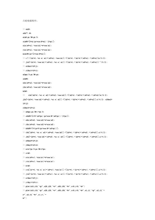
disp’******** 滚子摆动从动件凸轮设计********'disp '已知条件:’disp ’凸轮作顺时针方向转动,从动件做摆动’disp’从动件在推程作等加速/等减速运动,在回程作等加速等减速运动’rb=52;rt= 10;qm=15;ft= 60;fs=10;fh = 60;alp = 35;a=140;l=122;q0=asin(rb/a)*180/pi;fprintf (1,’基圆半径 rb =%3、4f mm\n',rb)fprintf(1,’滚子半径 rt =%3、4fmm \n’,rt)fprintf (1,' 起始角度q0= %3、4f mm \n’,q0)fprintf (1,'最大摆动角度 qm =%3、4fmm \n',qm)fprintf (1,'推程运动角 ft =%3、4f 度\n',ft)fprintf(1,' 远休止角fs = %3、4f 度 \n',fs)fprintf(1,' 回程运动角fh=%3、4f度 \n’,fh)fprintf(1,’推程许用压力角 alp=%3、4f 度\n',alp)hd= pi / 180;du = 180/pi; %角度弧度互换d1 = ft+fs;d2=ft + fs+fh;disp ' 'disp '计算过程与输出结果:’disp ’1-计算凸轮理论轮廓得压力角与曲率半径'disp '1-1 推程(等加速/等减速运动)'s=zeros(ft);ds = zeros(ft);d2s =zeros(ft);vt=zeros(ft);st1=zeros(ft);at=zeros(ft);at = zeros(ft);atd=zeros(ft);pt = zeros(ft);for f= 1: ftif f <=ft/ 2s(f)=2*(qm/ft^2)*f^2;st1(f)=s(f);s=s (f);%推程加速方程式ds(f)=(qm/ft^2)*f;vt(f)=ds(f);ds= ds(f);d2s(f)=4*qm/ft;at(f)=d2s(f);d2s=d2s(f);elses(f)=qm-2*qm*(ft-f)^2/ft^2;st1(f)=s(f);s=s(f);%推程减速方程式ds(f)=4*qm*(ft-f)/ft^2;vt(f)=ds(f);ds= ds(f);d2s(f)=-4*qm/ft^2;at(f)=d2s(f);d2s = d2s(f);endat(f)=atan((-l*(1-ds))/(a*sin((s+q0)*hd))—(-1)*cos((s+q0)*hd)/sin((s+q0)*hd));atd(f)= at(f) * du; %推程压力角得角度与弧度表达式p1= —a*sin(f*hd)+l*sin((s+q0-f)*hd)*(ds-1);p2= a*cos(f*hd)+l*cos((s+q0—f)*hd)*(ds-1);p3=—a*cos(f*hd)+l*(ds-1)^2*cos((s+q0-f)*hd)+l*d2s*sin((s+q0-f)*hd);p4=—a*sin(f*hd)-l*(ds-1)^2*sin((s+q0-f)*hd)+l*ds*cos((s+q0—f)*hd);pt(f)= (p1^2+p2^2)^1、5/(p1*p4-p2*p3) ;p =pt(f);endatm = 0;for f = 1 : ftif atd(f)> atmatm= atd(f);endendfprintf (1,'最大压力角 atm =%3、4f度\n',atm) for f =1 : ftifabs(atd(f) - atm) < 0、1ftm= f;breakendendfprintf (1,’对应得位置角 ftm=%3、4f度\n',ftm)if atm> alpfprintf (1,' *凸轮推程压力角超过许用值,需要增大基圆!\n')endptn =rb ;ftn=0;for f = 1: ftif pt(f)< ptnptn = pt(f);endendfprintf(1,' 轮廓最小曲率半径ptn = %3、4f mm\n',ptn) for f = 1 : ftif abs(pt(f) -ptn) 〈0、1ftn=f;breakendendfprintf (1,' 对应得位置角 ftn = %3、4f度\n’,ftn) if ptn〈rt + 5fprintf(1,'* 凸轮推程轮廓曲率半径小于许用值,需要增大基圆或减小滚子!\n’)enddisp ’ 1—2回程(等加速等减速运动)'s = zeros(fh);ds = zeros(fh);d2s=zeros(fh);ah = zeros(fh);ahd = zeros(fh);ph =zeros(fh);for f = d1: d2k =f—d1;if k<=fh / 2s(f) =qm—2*qm*(k)^2/fh^2;st1(f)=s(f);s= s(f);ds(f)=-4*qm*k/fh^2;ds =ds(f);d2s(f)=-4*qm/fh^2;d2s=d2s(f);elses(f) =2*qm*(d2—f)^2/fh^2;st1(f)=s(f); s = s(f);ds(f)=-4*qm*(d2—f)/fh^2;ds = ds(f);d2s(f)=4*qm/fh^2;d2s = d2s(f);endat(f)= atan((—l*(1—ds))/(a*sin((s+q0)*hd))-(—1)*cos((s+q0)*hd)/sin((s+q0)*hd));atd(f) = at(f) *du;%推程压力角得角度与弧度表达式p1= -a*sin(f*hd)+l*sin((s+q0-f)*hd)*(ds-1);p2= a*cos(f*hd)+l*cos((s+q0-f)*hd)*(ds—1);p3=-a*cos(f*hd)+l*(ds—1)^2*cos((s+q0-f)*hd)+l*d2s*sin((s+q0—f)*hd);p4=-a*sin(f*hd)—l*(ds-1)^2*sin((s+q0-f)*hd)+l*ds*cos((s+q0-f)*hd);pt(f)= (p1^2+p2^2)^1、5/(p1*p4-p2*p3) ;p=pt(f);endatm = 0;for f = 1 : ftif atd(f)〉 atmatm = atd(f);endendfprintf (1,' 最大压力角atm = %3、4f度\n',atm)for f = 1 : ftif abs(atd(f)- atm)< 0、1ftm = f;breakendendfprintf(1,'对应得位置角 ftm=%3、4f 度\n’,ftm)if atm〉alpfprintf(1,’ * 凸轮推程压力角超过许用值,需要增大基圆!\n')endptn = rb ;ftn=0;for f = 1 : ftif pt(f)< ptnptn= pt(f);endendfprintf (1,’轮廓最小曲率半径ptn = %3、4fmm\n',ptn) forf= 1:ftif abs(pt(f)—ptn) < 0、1ftn =f;breakendendfprintf (1,'对应得位置角 ftn = %3、4f度\n',ftn)if ptn< rt + 5fprintf (1,' *凸轮推程轮廓曲率半径小于许用值,需要增大基圆或减小滚子!\n')enddisp’2- 计算凸轮理论廓线与实际廓线得直角坐标’n = 360;s=zeros(n);ds = zeros(n);r = zeros(n);rp = zeros(n);x= zeros(n);y = zeros(n);dx =zeros(n);dy = zeros(n);xx= zeros(n);yy = zeros(n);xp= zeros(n);yp = zeros(n);xxp =zeros(n);yyp = zeros(n);for f =1: nif f <=ft/2s(f)=2*(qm/ft^2)*f^2;s = s(f);ds(f)=(qm/ft^2)*f;ds=ds(f);elseif f > ft/2 & f <= fts(f)=qm-2*qm*(ft-f)^2/ft^2;s = s(f);ds(f)=4*qm*(ft-f)/ft^2;ds= ds(f);elseif f > ft&f <=d1s = qm;ds = 0;elseif f〉 d1&f<= (d2-fh/2)k = f — d1;s(f)=qm-2*qm*(k)^2/fh^2; s = s(f);ds(f)=—4*qm*k/fh^2;ds =ds(f);elseif f>(d2-fh/2)&f<=d2s(f)=2*qm*(d2—f)^2/fh^2; s=s(f);ds(f)=—4*qm*(d2-f)/fh^2;ds =ds(f);elseif f > d2& f〈= ns = 0;ds = 0;endxx(f) = a*cos(f*hd)—l*cos((s+q0—f)*hd);x=xx(f);yy(f)=a*sin(f*hd)+l*sin((s+q0-f)*hd);y=yy(f);dx(f)=-a*sin(f*hd)+l*sin((s+q0-f)*hd)*(ds-1);dx = dx(f);dy(f)= a*cos(f*hd)+l*cos((s+q0—f)*hd)*(ds-1);dy =dy(f);xp(f) =x-rt*(dy/sqrt(dx^2+dy^2));xxp=xp(f);yp(f) =y+rt*(dx/sqrt(dx^2+dy^2));yyp=yp(f);r(f) =sqrt (x^2+ y ^2 );rp(f) = sqrt(xxp ^2 + yyp ^2 );enddisp ' 2-1推程(等加速/等减速运动)’disp ’凸轮转角理论x理论y实际x 实际y'for f = 10 :10 :ftnu = [f xx(f) yy(f) xp(f)yp(f)];disp(nu)enddisp ' 2-2 回程(等加速/等减速运动)'disp '凸轮转角理论x理论y实际x 实际y'for f = d1:10 : d2nu = [f xx(f) yy(f)xp(f)yp(f)];disp(nu)enddisp’2-3 凸轮轮廓向径’disp '凸轮转角理论r 实际r’for f = 10:10 :nnu= [f r(f) rp(f)];disp(nu)enddisp '绘制凸轮得理论轮廓与实际轮廓:’plot(xx,yy,'r—、') %理论轮廓(红色,点划线) axis ([-(150)(150)-(150)(150)])%横轴与纵轴得下限与上限axisequal % 横轴与纵轴得尺度比例相同text(50,0,’X')%标注横轴text(0,50,'Y’) %标注纵轴 text(-5,5,’O’)%标注直角坐标系原点title('摆动从动件盘形凸轮设计')% 标注图形标题hold on; % 保持图形plot([—(rb)(rb)],[00],’k’)%横轴(黑色) plot([00],[—(rb)(rb+rt)],’k’)% 纵轴(黑色)ct = linspace(0,2*pi); %画圆得极角变化范围 plot(rb*cos(ct),rb*sin(ct),'g’)%基圆(绿色) plot(xp,yp,'b’) %实际轮廓(蓝色)。