Fast UniFrac ,PCoA 分析软件使用说明
casp 说明
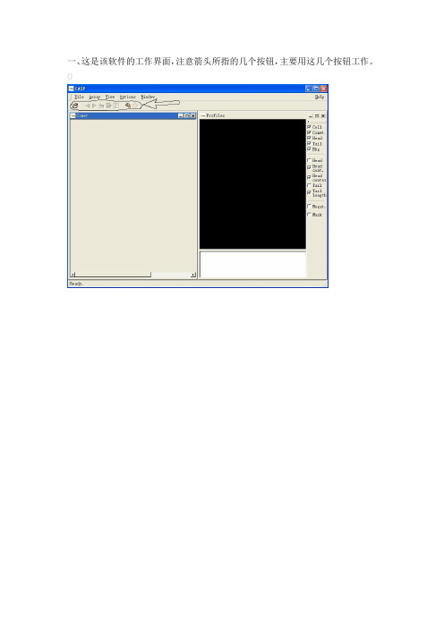
一、这是该软件的工作界面,注意箭头所指的几个按钮,主要用这几个按钮工作。
0二、单击红色箭头所指按钮,即打开文件,注意图像文件应是TIF格式,(蓝色圈定所指),按住SHIFT键,可以同时选定多个文件,点击OK,(绿色圈定),CASP软件就读入了您所选的图像文件。
三、点击view下拉菜单,选红色箭头所指的”result window",在分析后您就可以看到您的结果窗口,绿色箭头所指是我做的彗星图像。
四、下面就可以开始分析了,分析之前最好把右侧的head 和tail选中,(绿色箭头所指,这样可以出现头、尾分明的视觉效果,如图),在图像分析框内按住左键下拉,出现黄色箭头所指的框,这个框一定要圈住整个要分析的一个彗星图像,然后就是用到红色圈定区域的按钮了,我分别做了标号,逐一解释:1和2:可以选前或后面的图像进行分析,即上一个和下一个的功能,分析完第一个,当然要选下一个分析,很简单!!!3:这是分析的功能键,黄色箭头所指的框圈住彗星后,点击此按钮就可以分析了。
4:每分析完一个彗星后,都要点击一下它,它会把结果数据保存到结果窗口,点击后,它会变灰。
(这很关键)。
5:背景选择按钮,点击它,框的背景会上下变化,(注意黄色箭头所指的框,较小的框是背景框,较大的是工作框,这两个框在分析之前是可以调整的,一般工作框要大于背景框。
6:正式分析前一定要点击它,否则没有结果,如果不点击它,只是预分析状态,在这种状态下,可以把分析条件调好,然后进入正式分析,点击它后,此钮上会出现一斜杠。
(如图)。
蓝色箭头所指区域是分析后的曲线,主曲线是单峰,如果是双峰,就是凋亡细胞。
曲线图下面列举了几个数据,不全,全部结果在结果窗口。
(下图)五、分析过程中或分析完成后,都可以看您的result窗口,如图,将图像分析窗口最小化(红色箭头),就显示出结果窗口(绿色箭头),从左到右依次是文件名(name)和分析的各个指标。
六、分析完成后,别忘了输出结果,点file下拉菜单,选红色箭头所指区域的“输出结果”,将会出现第七步的图像。
Phoenix分析软件功能介绍 PPT

Thyoaunk
End
配置界面介绍
• 根据测试数据选择相应网 络制式
• 内容配置选择在报告中是 否显示参数覆盖、事件统 计
• 参数配置选择在报告中展 示的参数
• 事件配置勾选在报告中需 要统计的事件
• 阀值是报告中统计参数是 否合格的标准值
• 阀值条件是参数与标准值 的关系,满足该关系的参 数值统计为合格
• 累计方向是对各区间参数 采样点占比的累加方向。
区间、颜色编辑-生成报告
• 覆盖图、柱状图、表格信 息的勾选是在报告中展现 参数轨迹图、各区间占比 的柱状图、表格统计个区 间参数采样点和占比
• +号是添加参数区间、-号 是删掉参数区间
• 双击值和颜色两列都会弹 出范围编辑器,可对区间 范围及其颜色进行修改
• 配置完成点击保存更改, 另存为则可以把配置好的 模板导出来,方便其他人 导入
WCDMA参数窗口展示
• WCDMA参数 窗口展示当前扰码、LAC、CI,激活集 、监测集等小区集合;RSCP、EC/NO、Tx Power、 Bler、SIR等参数。
GSM参数窗口展示
• GSM参数 窗口展示当前小区LAC/CI/BCCH频点、信 号电平、语音质量、频段及其邻区的无线参数。
业务速率、经纬度
功能键可显示数据业务速率、经纬度 信息、室内/外地图窗口
• 功能键可 显示信令、 事件,可对 信令和事件 进行查找
• 查找出来的 信令和事件 与各参数窗 口关联,双 击查找到的 事件和信令 可在其他参 数窗口找到 对应的参数 值
信令和事件显示、查询
• 功能键可 对工作窗口 进行排列、 保存工作区 、加载工作 区
(un)WeightedUniFrac分析
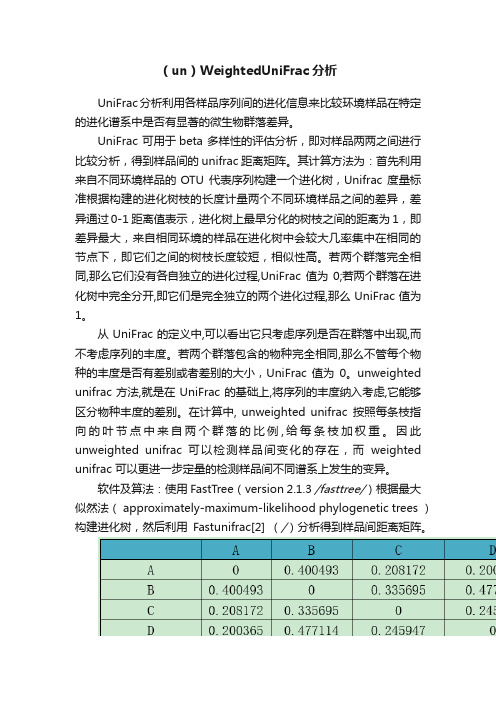
(un)WeightedUniFrac分析UniFrac分析利用各样品序列间的进化信息来比较环境样品在特定的进化谱系中是否有显著的微生物群落差异。
UniFrac 可用于beta 多样性的评估分析,即对样品两两之间进行比较分析,得到样品间的unifrac距离矩阵。
其计算方法为:首先利用来自不同环境样品的OTU 代表序列构建一个进化树,Unifrac 度量标准根据构建的进化树枝的长度计量两个不同环境样品之间的差异,差异通过0-1 距离值表示,进化树上最早分化的树枝之间的距离为1,即差异最大,来自相同环境的样品在进化树中会较大几率集中在相同的节点下,即它们之间的树枝长度较短,相似性高。
若两个群落完全相同,那么它们没有各自独立的进化过程,UniFrac值为0;若两个群落在进化树中完全分开,即它们是完全独立的两个进化过程,那么UniFrac值为1。
从UniFrac的定义中,可以看出它只考虑序列是否在群落中出现,而不考虑序列的丰度。
若两个群落包含的物种完全相同,那么不管每个物种的丰度是否有差别或者差别的大小,UniFrac值为0。
unweighted unifrac方法,就是在UniFrac的基础上,将序列的丰度纳入考虑,它能够区分物种丰度的差别。
在计算中, unweighted unifrac按照每条枝指向的叶节点中来自两个群落的比例,给每条枝加权重。
因此unweighted unifrac 可以检测样品间变化的存在,而weighted unifrac 可以更进一步定量的检测样品间不同谱系上发生的变异。
软件及算法:使用FastTree(version 2.1.3 /fasttree/)根据最大似然法( approximately-maximum-likelihood phylogenetic trees )构建进化树,然后利用Fastunifrac[2] (/)分析得到样品间距离矩阵。
Table(un)weighted unifrac distance matrix注:第一行和第一列均为样品。
环境微生物多样性分析

(((SEQ1:0.02120,(SEQ2:0.09111,SEQ3:0.04491)node1:0.00097)node2:0.0 0194, (SEQ4:0.03160,SEQ5:0.04378)node3:0.00365)node4:0.00188,SEQ6:0.00 881)node5:0.00739;
Muscle
/muscle/
/pynast/#
/fasttree/
Phylogenetic tree
NEWICK format:
NEWICK is a standard format that is recognized by most programs that generate or allow visualization of phylogenetic trees including PHYLIP, TREE-PUZZLE, ARB, and TREEVIEW.
unWeighted unifrac
Qualitative
Weighted unifrac
Quantitative
Unifrac分析软件
Unifrac /unifrac/index.psp
Mothur /wiki/Unifrac.weighted
/unifrac/
Distance Visualization
Nonmetric Multidimensional Scaling (NMDS)
Principal Coordinate Analysis (PCoA)
Hierarchical clustering
H2
Bacteroidetes Cyanobacteria Spirochaetes
顶刊16s扩增子测序数据分析流程

顶刊16s扩增子测序数据分析流程下载温馨提示:该文档是我店铺精心编制而成,希望大家下载以后,能够帮助大家解决实际的问题。
文档下载后可定制随意修改,请根据实际需要进行相应的调整和使用,谢谢!并且,本店铺为大家提供各种各样类型的实用资料,如教育随笔、日记赏析、句子摘抄、古诗大全、经典美文、话题作文、工作总结、词语解析、文案摘录、其他资料等等,如想了解不同资料格式和写法,敬请关注!Download tips: This document is carefully compiled by theeditor.I hope that after you download them,they can help yousolve practical problems. The document can be customized andmodified after downloading,please adjust and use it according toactual needs, thank you!In addition, our shop provides you with various types ofpractical materials,such as educational essays, diaryappreciation,sentence excerpts,ancient poems,classic articles,topic composition,work summary,word parsing,copy excerpts,other materials and so on,want to know different data formats andwriting methods,please pay attention!顶刊16S rRNA扩增子测序数据分析流程详解在微生物生态学研究中,16S rRNA基因扩增子测序是一种常用的技术,它能有效地揭示样本中的微生物群落结构和多样性。
微生物16S测序数据的正确打开方式

微生物16S测序数据的正确打开方式16S rRNA基因测序(也称16S rDNA测序)是最常用的菌群多样性分析的手段。
对于新手,如果收到一份不讲“人话”的16S测序分析报告,很快就会被各种生态学术语、各种指数、各种分析方法弄晕。
7个问题串起16S测序的核心结果怎么办?用你的研究逻辑来梳理16S测序数据(图1)。
简单地说,做16S测序是为了鉴定样本中的微生物(细菌)群组成,找微生物群与疾病或表型的相关性。
详细地说,1)首先想了解在不同组样本中各有哪些微生物存在和丰富度(对应于菌群鉴定和α多样性分析);2)接着想看不同样本组间微生物群组成是否存在差异(对应于β多样性分析);3)如果是,那么就有必要找出引起不同组样本微生物群差异的关键菌。
如果不是,那说明微生物群比如肠道菌群与疾病或表型可能并不相关(基于已有的研究,这种可能性比较小);4)找到了关键菌,在临床上,很自然会想到,这些(个)关键菌是否可以作为Biomarker(对应于疾病诊断模型构建),比如用于区分糖尿病前期患者与健康组的标志物;5)以及这些(个)菌是否与临床指标具有相关性(对应于菌群与临床指标的相关性分析);也会进一步想到,既然不同组的微生物群落存在差异,又与疾病具有相关性,6)那么这些菌群是如何影响宿主的,可能参与了哪些代谢途径(对应于菌群基因功能预测);7)这些预测到的菌群功能是否与疾病有关,通常是肯定的。
最后把这些结果整合起来分析,可以初步得出菌群组成的变化是如何与疾病或表型相关的。
顺着上述7个生物学问题来看16S测序结果,你会轻松拨开迷雾,直达核心结果。
图1 7个问题串起16S测序的核心结果6张图就够发菌群与疾病相关性文章编者对2019发表的数十篇以16S测序为主的肠道菌群与疾病关系研究文章(IF 5至10分)的内容进行了分析和归纳,发现大部分文章的Results部分都是由图1所列的核心结果组成。
以联川生物医学16S测序报告为例,具体讲解16S测序文章中的核心结果及其对应的图表。
CFAST使用指南中文
程序简介1.1起步1.1. 1学习使用FAST1.2. 2硬件及软件配置1.1. 3安装1.2. 软件概述及适用范围1.2.1火灾模型的实用性1.2.2火灾1.2.3羽流及Layers1.2.4出口风流1.2.5热传导1.2.6物种浓度与密度1.2.7软件使用假设与范围1.3什么是用户使用界面(GUI)?1.3.1使用鼠标及其它定点设备1.3.2 GUI的有关术语1.3.3GUI界面按钮及菜单项1.4启动FAST1.5FAST主菜单2 创建程序输入数据2.1创建一新输入文件一实例2.2基本的火灾模型输入2.2.1输入输入文件的文件名2.2.2记录时间及电子表格输出2.2.3设置试验环境2.2.4定义若干空间结构2.2.5定义水平流之间的联系2.2.6定义竖直流之间的联系2.2.7增设水喷淋器和火灾探测器2.2.8定义火源2.2.9记录与时间相关的火灾实验曲线2.2.10工具集2.3高级火灾模型输入方法详解2.3.1建筑空气控制系统HV AC2.3.2HV AC系统通风口2.3.3HV AC系统内部连接与安装2.3.4HV AC系统通风管道2.3.5HV AC系统通风机2.3.6顶棚射流表面的选取2.3.7指定多个火源2.3.8顶棚到地板的热传导2.3.9定义目标层2.4交互式数据库2.4.1选取默认材料2.4.2选取默认对象2.4.3创建变换的数据库2.4.4编辑热物理数据库2.4.5编辑对象数据库对象火灾曲线61对象备注63闪火传播对象属性642.5修改配置文件2.6运行一个简单实例2.7新文件定义的标准过程2.8数据文件的打开和保存2.8.1选取一个已有的数据文件2.8.2创建一个新的输入数据文件2.8.3保存对数据文件的修改3运行火灾模型3.1进行模拟3.2边模拟边运行3.3处理模拟过程中的事件3.4保存模拟出的模型4复杂模型实例4.1事件4.2计算机分析4.3输入数据4.3.1输入文件名4.3.2定义外部条件4.3.3指定模拟时间和电子表格的输出4.3.4改变火灾房间的几何形状4.3.5改变通风口4.3.6改变火源的定义4.3.7保存对数据文件的修改4.4运行模型4.5模型运行结果5预测软件包5.1逃生时间5.2喷淋器与探测器的动作5.3房间烟气温度5.4上浮的热气压头5.5顶棚射流温度5.6顶棚羽流温度5.9通过开口的质量流5.10 羽流充填速率5.11辐射引燃5.12开口处的烟气流动5.13托马斯轰然公式5.14通风极限6 文件操作6.1改变路径6.2改变显示单位6.3设置色制和模式6.4输入数据的纠错6.5拷贝文件6.6打印文件6.7浏览文件6.8删除文件7 参考文献及附录文献信息FAST是一本有关火灾模型的使用工具手册他参考了以前的火灾模型CFAST并且增加了火灾形成过程提供了在分隔空间构筑物中的火现象的工程计算这本使用手册提供了使用范例及相关的资料详细介绍了软件的安装方法及使用指南关键词计算机模型计算机程序排空火灾模型火灾研究火险评价人的行为毒性订购信息美国NIST研究所FAST用户指南预测火灾发展与烟气蔓延的工程工具建筑火灾研究实验室美国NIST研究所简单的代数方程是工程计算的基础1984年Bukowski提出了用一系列独立的火灾计算来评估一个复杂,交互的过程,即,火危险分析[ 1 ]在1985年一系列适用于火灾评估的方程出版发行了尼尔森[ 3 ] 用 FIREFORM 和 FPE工具进一步扩展了这个概念并且提供了一广泛地在火灾安全工程计算中被使用的软件包这个软件包里提供了简单的工程计算模型1989年6月NIST研究所的火灾研究中心现BFRL的一下属机构针对火灾对居民人身安全的危害以及室内家具电线等物品的火灾时的相关危害发布了一种定量分析的方法这种分析方法经过6年的深入研究最终推出了第一代应用软件HAZARD I它是世界上第一代火灾模拟综合应用软件它结合了专家们的判断和计算的标准来评估一次特定火灾的后果FAST是建立在CFAST基础之上的一种程序集他提供有关框架结构的火险工程评估他是继HAZARD I 和FASTLite之后的应用在火险计算上的第二代软件FAST包括了以前FIREFROM中的独立的工程计算,是CFAST它包括了HAZARD I和FASTLite的更新版本他的用户界面与FASTLite相似本说明书提供了参考文献和应用实例以及使用指南说明了软件的安装等操作首先注意一点fast是针对火灾安全领域的专业人士设计的并且是对他们决策的补充软件的目的是对火灾灾害结果提供定量分析该模型只能在对计算的精确性进行证实性测试后在其允许的误差范围内使用然而正像许多其它计算机软件那样软件使用者提供的输入数据直接决定了计算结果的准确性如果有模型得到的预测结果精确性较差有可能导致错误的结论所以又该模型得到的所有结果都应该凭一般经验进行审核11开始FAST是建筑火灾蔓延的预测工具这张光盘中包括该软件及相关文件用户可按照说明书进行安装虽然该软件的安装及运行较简单但是要想更有效的使用该软件的各项功能用户必须阅读使用说明建议浏览一下软件使用说明书的目录熟悉该使用手册的内容1.1.1学习使用 FAST为典型火灾案例的现实模拟量建立恰当的输入数据的过程是比较复杂的当用若干典型参数来描述现实模拟量时几乎所有特定测试实例的数据都能被定制本使用说明中包括了所有的数据输入的详细描述这一节提供了一个可能的方案指导用户使用1第5页的1.2节对FAST的理论基础及预测方程使用的限制条件进行了概述2从第14页开始对用户界面中的每一项内容进行了详细的描述如鼠标键盘的使用数据输入界面及结果显示画面初学者有必要对本章进行学习以便熟悉图形用户界面的一些概念3在第23页的第2节介绍了一个单室火灾的简单范例提供了运行该实例的具体步骤学习本范例后用户将熟悉软件的基础操作4在第83页的第5节讲述了许多预测工具它们都包括在FAST软件中能用来对个别的火灾现象进行描述这些工具需要两个以上的输入参数大多数的程序只需要做相对较少的工作就可获得预测结果5最后在第25页第2.2节对FAST的数据输入进行了详细的描述它可用来定制个别测试实例的数据1.1.2硬件及软件配置要求1.1.3软件安装安装向导提示了必要的信息并拷贝必要的文件到硬盘上FAST是基于DOS环境下的程序应直接在DOS环境下安装如有必要在安装前可退出Windows环境及应用程序以下是安装步骤将安装光盘放入光驱输入如下命令D:INSTALL在安装的过程中有几个问题需要用户回答可根据自己的需要做适当的回答一般都是取默认值在每一个安装画面中安装向导都有相应的提示下面对安装步骤进行具体介绍将fast单独安装在一个目录中开始的两个安装画面显示了主程序的安装目录一般缺省为c安装程序至少需要12兆直接的空间当程序拷贝时安装向导将显示出安装进度为了能正确安装安装组件可能需要创建或是移动DOS中的启动文件CONFIG.SYS中的语句FILES=如果你要手动移动你可以跳过这个步骤FILES=语句至少要为该软件指定50个文件1. 2概述与局限预测火灾趋势的分析模型从60年代就开始发展经过30多年的发展与完善模型已相当成熟起初研究的重点是用数学语言描述火灾发展的三个阶段即发展蔓延熄灭这种与实际分离较大的数学表达方式仅为安全性分析提供了火灾燃烧现象的一小方面特征根据多重的单个现象的组合可以编制出复杂的计算机程序给出输入参数后就可以预测出预计火灾发生的原因这些分析模型经过发展已可以给出最符合工程实际应用的火灾状态的预测当前国际上已有36种火灾模型其中20种是预测火灾发生的环境温度19种预测烟气运动6种计算火灾的发展速率9种预测材料的耐火性4种计算火灾探测器与水喷淋器的灵敏度2种是计算火灾中人员疏散时间现在这些计算机模型在使用范围复杂程度使用目的等方面变化很大如单室火灾模拟程序ASET移植性很好对于单个房间内的火灾可给出较好的预测有些模型为了特定的使用目的提供了单一的功能如COMPF2程序计算发生跳火的房间温度LAVENT程序计算在一设有水平出口和风流减速帘的房间内顶棚射流的相互作用此外还有HARVARD 5 code 和FIRST用来预测单一房间内多个燃烧体的燃烧状态除了上面提到的单室火灾模拟程序外还有一些多室火灾模拟程序包括BRI HARVARD 6 code FASTCCFM CFAST 和 FASTLite所有的火灾模型都可分为两类一种是根据质量守恒动量守恒和能量守恒等基本物理定律建立的一种是根据实验做出曲线来找出个参数之间的关系这两类模型中都采用了数学近似及简化假设根据火灾的物理原理可建立数学表达式再将得出的守恒方程式代入温度烟气浓度等参数的预测方程并输入计算机就可得到解决方案发生火灾的环境是不断变化的所以这些方程通常为微分形式一个完整的方程组能计算出在一定时间内受限空间的火灾环境火灾模型假定在任何时候控制体内的温度烟气密度组分浓度等参数都相同不同的火灾模型将建筑物划分为数目不同的控制体目前应用最广的一类火灾模型称为区域模型通常它把房间分为两个控制体即上部热烟气层与下部冷空气层在发生火灾的房间里把火羽流或顶棚射流当作附加控制体可提高预测的准确性这种分层的方法来自对火灾实验的观察热烟气在顶棚聚集并从顶棚开始充满整个房间在实验中层中环境是不断变化的而两层厚度的变化更大所以区域模型在大多数火灾环境中可得到相当接近现实的模拟此外还有网络模型和场模型前者把每一间房间看成一个节点来预测远离起火房间某地点的环境而场模型则完全从另一个角度出发它把一个房间划分为上千甚至是上百万个网格它们能够用来预测层内的环境变化但是其运行时间大大超过区域模型所以只在细节计算中使用1.2.1 火灾模型的适用性在FAST中使用的CFAST模型是用来计算火灾期间建筑物内的烟气及温度的分布CFAST是基于解状态参数方程组的基础上的这些参数压力温度等是基于在一微小时间间隔内的焓与质量变化之上的这些方程式根据能量守恒质量守恒动量守恒以及理想气体定律而得到的这些守恒方程式是绝对正确的所以有火灾模型得到的错误结果只会是由方程的数学表达式及简单假设造成的上正确的限制条件用户应熟悉模型所遵循的火灾物理原理文献中提供的典型应用实例以及模型使用的限制条件1.2.2火源在CFAST中火源简化为一种以确定速率不断放热量的燃料通过燃烧,燃料的燃烧热转换为热焓l同时根据特定组分的产生率转化为该组分的质量在羽流和顶棚射流中也可以发生燃烧对手不受限火源燃烧将全部在羽流内进行对于受限火源燃烧可在任何有足够氧气的地方发生当一定的氧气被卷吸到火羽流中与未完全燃烧的燃料同时进入上部烟层上层内就可以发生燃烧接着是门道射流第二个房间上层第二个房间门道第三个房间上层直到燃料完全消耗或排到室外为止新版的CFAST可以在若干个房间中逐一监测多个火源这些火源全部作为分离的实体处理就是说它们与羽流没有相互作用与房间壁面之间没有辐射换热CFAST在计算火区增大时没有考虑燃料的热解模型因此设定火源与真实火源的相似程度如何将决定计算结果的准确性1.2.3羽流与气层在任何正在燃烧的物体上方都会形成羽流它不是任意气层的一部分但却是能量和质量由下层向上层输送的驱动源CFAST不使用点火源来近似羽流而是用经验公式决定由羽流引起的层间质量转移在不同层和不同房间之间能量和质量传输主要有两种形式一种是着火房间内的羽流另外一种是出现在门窗开口处的混合源在计算刚开始时室内每层的状态都与环境相同但为了避免计算中出现数学问题程序中预先假设上层的体积为房间体积的0001随着焓与质量由羽流送入上层上层体积开始膨胀层界面向下移动只要界面尚未到达开口的上缘就不可能有通过开口的流动在火灾的这种早期阶段上层气体的膨胀将使下层空气由开口流进相邻的房间一旦界面低于开口的上缘便开始形成门道羽流(也有人称为门道射流)随着烟气由起火房间流入相邻房间后一房间的下层空气受到挤压于是一部分空气可沿开口下部返流入起火房间在这种门道羽流中气体混合在流入与流出的逆向流边界上进行决定开口流动也按羽流处理不过这两者对空气的卷吸方式有差别因此直接使用羽流的计算方法会产生一些误差上述流动都是由压力差和密度差引起的而这两者又是由温度差和气层厚造成的因此得到正确流动的关键是在各层之间恰当分配来自火源的质量和焓1.2.4开口流开口流是火灾模型的控制现象因为它的波动很快并可在所有源项中迅速输送大量的焓开口流可分为水平流动和竖直流动两种类型前者如通过门窗的流动后者指的是流过房间顶棚或地板开口的流动对于火灾环境迅速变化的情况竖直流动很重要竖直流动不完全由上下气体的密度差决定还受气体的体积膨胀影响除了快速膨胀情况之外这种压差很小往往忽略不计但是若需了解小压差下的流动例如机械通风系统中产生的流动那么这种压差就变得很重要了大气压约为100,000Pa,火源产生的压力变化范围为11000h而机械通风系统产生的压差约为1100h为了正确解决它们的相互影响从问题整体来说应当能在100,000Pa的压力范围内考虑约01Pa的压差1.2.5传热在气层与房间壁面之间存在对流换热而墙壁顶棚和地板又以导热形式向外传热CFAST允许每个房间的墙壁地板和顶棚使用不同的材料但各个部分所用的材料性质应当相同同时每种壁面可分为三层按这些层分别进行导热计算,这有助于用户处理实际建筑物的结构材料的热物性是随温度改变的不过在通常的火灾温度范围内大多数物体的热物性变化不大因此在CFAST中将它们取为常数在火源气层和房间壁面之间还存在辐射传热其传热速率是温度差气体与壁面辐射率的函数火源和典型壁面间的辐射率变化很小气层的辐射率却随其组分浓度变化烟气中的颗粒C02水蒸气都是强辐射体因此组分浓度的误差将引起焓在不同层内分布的误差并由此而导致温度误差和流动误差1.2.6组分浓度模拟计算开始时各层的初始条件与环境相同初始温度由用户指定氧气和氮气的质量分数分别为23和77水分用相对湿度表示也由用户指定其它组分的浓度为零但随着燃料的热解多种组分开始生成质量并了解每层体积随时间的变化质量除以体积便是质量浓度将其与分子量结合起来又可得出体积百分比浓度或ppm浓度由此可见CFAST模型相当全面地考虑了物理化学流体流动与传热等方面在有些情况下可以直接使用质量能量和动量的基本定律但很多其它场合下必须使用经验公式乃至合理猜测来弥合现有知识的不足这些必要的假设可能会导致结果的不确定因此用户应当清除程序原有假定和局限性谨慎使用程序计算包括对关键参数取值范围的敏感性分析以便能够对结果的不确定性作出估计1.2.7假定与限制1.3什么是图形用户界面(GUI)?FAST的界面是普通的图形用户界面图形指使用直线矩形颜色阴影来表示出三维图形界面大多计算机操作人员一般都熟悉MS-WINDOWS界面FAST的界面具有WINDOWS应用程序的特征但它却不是一个WINDOWS的应用程序它是用DOS命令来启动的1.3.1使用鼠标或其他定点设备定点设备诸如鼠标轨迹球等是在GUI可视化应用程序中常用的手动设备本软件有三种鼠标操作方式单击双击拖动1.3.2GUI使用术语图形用户界面的设计可支持多个应用程序的同时运行程序有桌面窗口和标题栏在程序窗口左上角的一小方框内有一小横杠点击它可拖动窗口或双击关闭窗口在FAST界面中使用了两种类型的窗口最常用的是对话窗口用户在对话窗口中输入数据然后点击窗口下方的一排按钮确认或否定窗口中显示的数据上图就是一对话窗口的实例当对话框弹出后用户必须处理完对话窗口中的数据后才能对其他窗口或菜单进行操作对当前输入值点击OK Cancel或Esc进行确认或否定浏览窗口是作为图形用户界面的背景窗口用来概述地显示已输入的参数值在FAST中最常用的是火灾脚本浏览窗口用鼠标点击窗口的标题栏可拖动浏览窗口在图形用户界面中有若干数据栏它可显示信息也可供用户输入数据在FAST中不同类型的数据栏中可显示特性曲线及相关函数用户可参考本节的详细介绍已确定selectability, functionality,并且显示特性曲线在选择数据栏时按Tab键可选择下面的或右边的为当前数据栏按Shift+Tab键可选择上面的或左面的为当前数据栏当然用户也可用鼠标来点击选择下面就见介绍FAST界面中的各类型的数据澜标签用于提示用户输入参数的类型它没有外框并且是黑色字体弹出一红色的错误提示窗口用户必须纠正后才能进行下一项的输入这两个按钮用来确认或拒绝输入值或为相关的输入打开一个附加窗口当用鼠标单击或按Tab键移至到所选位置后按Enter键后相应的功能就会实现下拉选框它提供了用户所有可选择的输入项图标它使用了图形按钮来表明了每一个按钮的功能选择列表它提供了一个参数列表在列表中只能选择一个输入项当前选择项用蓝底白字标明而其它待选项用白底绿字表示可通过鼠标双击来选择输入项滚动条有时当窗口尺寸不够显示信息时一个垂直或水平滚动条会出现在窗口右边或下边以便用户调节并显示出别的信息编辑表它是一种电子表格蓝底白字在窗口底部有输入值的范围提示输入范围由单元格内的输入数据决定只有当程序确定输入值有效时用户才能跳到下一单元格进行输入单元格的选择用 来控制光标与指针I 与 是图形用户界面中两种常用的定位标识1.3.3图形用户界面中的菜单菜单提供用户选择各种功能及应用程序点击图标后就会弹出相应的菜单FAST的用户界面提供了3种菜单桌面菜单文件菜单及软件包菜单桌面菜单提供用户选择FAST的其他程序模块它可在桌面上弹出也可从火灾方案浏览窗口中点击桌面图标以显示出桌面菜单在下面1.5节中将对各菜单项详细介绍文件菜单中Save和Save As选项用来保存数据文件用户可在火灾方案浏览窗口中点击标题栏或磁盘图标就可弹出该菜单该软件包提供了几种快速计算程序可在桌面菜单种选择tools项或点击工具箱图标弹出该菜单在后面第5章中将有详细介绍cd \FASTFAST按回车键后FAST的启动窗口将显示在屏幕上按回车键后可显示出桌面菜单第一次运行程序时用户可以自定义各参数的单位所定义的一组参数将在以后的计算中使用如在本手册中通常使用了公制单位如温度压力长度能量能量释放率能量吸收率质量及时间分别使用了摄氏度帕米焦耳千瓦瓦千克以及秒作单位若要修改单位设置可点击下拉菜单选择列表中的单位例如温度单位的下拉菜单选项由开尔文摄氏度Rankine华氏温度点击桌面菜单选项Options再点击User Specified Units单位设定窗口就会显示1.5 FAST组件概述FAST是由几个互相依存的分析模块组成的 上面讨论的桌面菜单依据工作类型及典型的命令把这些模块编排在一起供用户选择运行点击Fil e将出现二级菜单Open / New Database选择Database可查看修改或选择关于热物性的交互式数据库Run的二级菜单项有Run Fire Mode l和Analyze Result s前者用来计算火灾和烟气的特性后者用于对计算结果提供几种解释选项以做进一步分析并且保存结果Tools提供几种快速计算工具计算出火灾的特性曲线如轰然和通过出口的质量流等事件Option s用来定制FAST程序组Utilities查看拷贝打印数据文件Hel p提供FAST主程序窗口中每一个图标的概述及版本信息和联系电话2. 创建FAST程序的输入数据FAST是一种交互式界面友好的用于创建输入数据文件运行CFAST模型的应用程序在本使用说明中要描述该程序的所有功能是比较困难的用户最好是通过使用来学习它这一节将详细描述FAST中所有窗口中的具体内容另外用户必须在熟悉图形用户界面GUI的基础上再学习本节内容2.1创建一个新的输入文件介绍一个简单的实例为了帮助初学者熟悉FAST的基本操作本节提供一简单的使用实例包括详细的软件使用命令为了便于说明我们对一两室火灾进行了模拟两间房间及房间与户外都有一扇门火源为居民家庭中常见的易燃品进入FAST的目录键入如下命令就将启动FASTCD\FASTFAST如果是第一次启动FAST需要对各参数单位进行初始化在FAST启动画面出现后程序主画面将出现用鼠标点击File New开始定义一新的火灾方案起初有两个步骤即对建筑物进行几何描述指房在点击New之后建筑结构选择窗口将出现在这个窗口中用户可定义房间数量及构造本节选择了2个房间的实例并定义了房间的尺寸为2.4米宽 3.6米深 2.4高确定完建筑结构之后还要对火源进行定义对于一大范围的火灾火势的发展可以用以下关系式来准确表述这里Q表示释热速率表示火灾强度系数t表示时间在三种火灾强度分别为600s300s150s75s达到1055KW1000 BTU/s我们分别称为慢速中速快速特大火灾它们对于火灾探测系统的设计都具有指导作用相应的这些火灾增长曲线都有通用的防火程序支持本例中用了一中等速度与T2成正比发展的火灾实例在若干可燃物中只要没有特别易燃的可燃物一般选择中速曲线用上文介绍的方法选择两个房间的建筑结构用鼠标点击Medium Growth图标点击OK之后关闭窗口一个新窗口将出现用来定义火灾曲线的时间本例中的默认值为300秒和900秒点击OK后关闭窗口2.2基本火灾模型参数的输入当一个文件建立或打开将出现火灾方案预览窗口该窗口能使用户在运行模型之前浏览文件的主要特征用户还能定义建筑物的房间数起火房间数红色方格表示配有喷淋器及探测器的房间数蓝绿色方格由于当前的CFAST模型主要是用来计算房间之间的烟气流动而不关心建筑物内实际的房间结构所以不必在意窗口中的房间模型与实际情况是否接近火灾方案预览窗口分为3个部分上部为标题栏第二部分是关于房间房间之间的烟气流动喷淋器及探测器的布置火灾曲线的定义最后一部分提供了运行火灾模型所必需的背景信息如外部条件文件名和输出时间等每部分具体的输入方法介绍如下在浏览窗口的第一部分每一个文件都有一独立的内容描述在窗口中部即建筑结构浏览部分显示了当前已定义的房间数目在每一个表示房间的小方格内都有标注说明了水平开口与垂直开口的数目如门和窗开口在数量后加标识H屋顶或地板上的开口在数量后加标识V起火房间用红色方格表示配置了喷淋器及探测器的房间用蓝绿色方格表示放置有其它可燃物的房间用黄色方格表示在激活建筑物结构部分的图标之前必须先选择一房间结构以决定该图标命令执行的方式点击输入文件中的#1房间然后点击它的图标这时#1房间的大小和建筑材料就将显示点击Cancel关闭此几何窗口再点击。
数据分析软件使用说明书-MizoueProjectJapan

数据分析软件使用说明书数据分析软件使用说明书目录目录前言关于商标 (1)免责事项 (1)安装软件 (2)基本操作启动软件 (4)软件画面的说明(主画面) (5)读取数据文件 (6)显示数据文件的属性 (8)数据的再生・滚动操作 (10)使用波形显示 (12)使用光标 (13)使用触发检索 (15)关于预触发数据 (22)运算功能使用FFT・频谱图 (23)使用IFFT(逆FFT) (25)使用X-Y显示 (28)使用自动测量功能 (29)实用程序功能CSV(逗号分隔型取值格式)文件的输出. 30使用打印功能 (33)更改语言设置 (35)规格操作环境 (36)MIZOUE PROJECT JAPAN with RORZE1数据分析软件 使用说明书前言关于商标Microsoft 、Windows 是美国Microsoft Corporation 在美国及其他国家的注册商标或商标。
Windows 的正式名称为Microsoft Windows Operating System 。
Pentium 、Core Duo 、Core 2 Duo 、Atom 、Core i3、Core i5、Core i7是在美国及其他国家的Intel Corporation 或者其子公司的注册商标。
免责事项由于本产品及附带软件的使用或不能使用而对客户或第三方造成损害时,MIZOUE PROJECT JAPAN 有限会社以及RORZE 株式会社(以下称本公司)恕不负责,敬请谅解。
另外,由于客户的疏忽、无视注意事项及警告事项的不正常使用以及自然灾害造成的损害,本公司不承担法律责任,即使事先得到了关于以上危险的通知,也恕不承担责任。
使用说明书中所登载的PC 画面有时与实际画面不同。
并且,恕不进行关于登载错误等的赔偿,敬请谅解。
前言MIZOUE PROJECT JAPAN with RORZE2数据分析软件 使用说明书安装软件软件的安装将安装用光盘放入CD-ROM 驱动器中。
Rsoft软件说明介绍和使用

目录Rsoft简介 (3)Chapter 7 Tutorials 第七章教程 (5)Tutorial 1: Ring Resonator 教程1:环形共振器 (5)Device Layout: 器件结构: (5)Defining Variables 定义变量 (6)Drawing the Structure 画器件结构图 (6)Checking the Index Profile 核对折射率分布 (9)Adding Time Monitors 添加时间监视(探测)器 (10)Simulation: Pulsed Excitation 模拟:脉冲激发 (12)Launch Field 激发场 (12)Wavelength/Frequency Spectrum 波长/频率光谱 (12)Increasing the Resolution of the FFT 提高FFT的分辨率 (14)Simulation: CW Excitation 模拟:连续激发 (16)Tutorial 2: PBG Crystal: Square Lattice 教程 2:PBG 晶体:四方晶格 (17)Lattice layout 晶格布局 (17)Base Lattice Generation 基准晶格的创建 (17)Lattice Customization 定制晶格 (18)Checking the Index Profile 核对折射率分布 (18)Inserting Time Monitors 插入时间监视器 (19)Launch Set Up 激发场设置 (20)Simulation 模拟 (21)Data Analysis 数据分析 (22)Switching Polarization 改变偏振为TM模 (23)Periodic Boundary Condition Set Up (24)Tutorial 3: PBG Crystal: Tee Structure 教程 3:PBG晶体: T型结构 (24)Tutorial 4: PBG Crystal: Defect Mode 教程四:PBG 晶体:缺陷模型 (24)Rsoft简介包括BeamPROP、FullWAVE、BandSOLVE、GratingMOD、DiffractMOD、FemSIM, 以及MOST软件。
Fracpro-PT+10

Fracpro-PT 10.2中文版培训教材中国重庆2005年5月23日~28日中国石油勘探开发研究院采油工程研究所FracproPT 入门辅导前言在线帮助中包含大量的入门辅导以及你在运行 FracproPT 四个不同方式中的每一个方式时的使用实例。
该入门辅导的目的是使用户熟悉该软件各种各样的功能。
虽然我们推荐按照给出的入门辅导顺序进行学习,但是他们都是相互独立的。
如果你确信已经掌握了 FracproPT 的某一章,那么你可以跳过该章的入门辅导。
你还应该注意到:因为这些入门辅导是相对独立的,所以在使用 FracproPT 的公用模块时的说明往往会重复。
当你开始入门辅导的任何一章的学习的时候,你应该保存你的工作到磁盘。
我们建议你:重新命名对你来说包含富有意义的某些东西的文件。
如果时间不允许你运行到(该章节的)结束的话,那么,这将允许你返回到在入门辅导(的相应章节)中的相同的位置。
当然,你采用初始文件重新来一遍也是允许的。
目录第一章压裂分析方式1.1、根据设计参数来运行1.1.1 根据设计参数来运行1.1.2 查找输入文件1.1.3 压裂分析选项1.1.4 井筒结构1.1.5 储藏参数1.1.6 压裂液和支撑剂的选择1.1.7 施工泵序一览表1.1.8 压裂分析的控制1.2、使用服务公司的压裂数据1.2.1 用ASCII 文件创建数据库文件1.2.2 输入文件的选定1.2.3 输出文件的定义1.2.4 生成输出文件1.3、测试压裂的拟合1.3.1 测试压裂的拟合1.3.2 查找输入文件1.3.3 压裂分析选项1.3.4 模型的信道输入1.3.5 管柱工具结构1.3.6 储藏参数1.3.7 压裂液和支撑剂的选择1.3.8 施工泵序一览表1.3.9 压裂分析的控制1.3.10 压裂分析的讨论1.3.11 闭合应力的确定1.3.12 确定摩阻损失1.3.13 拟合净压力的大小1.3.14 拟合净压力下降的斜率1.3.15 保存测试压裂的拟合结果1.4、拟合主压裂施工1.4.1 拟合主压裂施工1.4.2 查找测试压裂拟合的输入文件1.4.3 修改测试压裂拟合的输入文件1.4.4 净压力拟合1.4.5 保存压力拟合结果1.4.6 生成报告1.4.7 在拟合中可能出现困难的原因第二章压裂设计优化2.1 背景2.2 第一步: 加载FracproPT 输入文件2.3 第二步:回顾必要的输入数据2.4 第三步: 选择压裂液和支撑剂2.5 第四步: 施工选择2.6 第五步定义经济优化2.7 第六步: 完成最终施工设计第三章产能分析入门辅导3.1 产能分析入门辅导背景3.2 第一步: 加载和更新产能分析的输入文件3.3 第二步: 预测生产效果3.4 第三步: 加载实际的生产数据3.5 第四步: 拟合实际的生产数据第四章编辑数据库4.1 编辑数据库第五章测试压裂分析辅导5.1 测试压裂分析第一章压裂分析模块综述本入门辅导将带领你通过 FracproPT 压裂分析方式中所用到的基本操作。
pcev20电脑元素仪软件使用说明

PCE 电脑元素分析仪软件使用说明1安装pce使用pce之前,必须首先安装pce软件。
1.1硬件和系统的最低要求为了运行pce,必须在计算机上安装相应的硬件和软件。
这些系统要求包括:.Microsoft Windows98 或更高版本操作系统。
.PII或更高处理器。
.至少1000M B硬盘安装空间。
.一个CD驱动器。
.Microsoft Windows支持的VGA或分辨率更高显示器。
.至少64 M RAM。
.至少一个RS232串口。
.鼠标或其它定点设备。
1.2安装pce软件步骤(1)将PCE的安装盘放入CD-ROM(2)运行光盘根目录下的可执行文件SETUP.EXE(3)选择文件的安装目录c:\program files\pce(4)安装程序组选pce(5)执行安装(6)安装成功会有提示2启动pce连接好串口线,打开下位机电源,执行pce,弹出pce测试界面如图-1:图-1在测试界面左下角第一个状态栏中显示串口打开状态,若串口打开失败,请检查串口是否被WINDOWS其它应用程序使用。
在测试界面左下角第二个状态栏中显示串口每次发送状态,若串口发送失败,请检查串口是否被WINDOWS其它应用程序使用。
在测试界面左下角第三个状态栏中显示串口接收通道电压状态,0v-4v接收电压正常,其它情况电压溢出,溢出时将不刷新A,T,C值。
3测试界面相关说明3.1通道参数显示图2系统按通道分别显示和操作,每个通道参数显示分为四个文本显示框和一个参数显示栏:文本显示框:(1)元素符号,当前测试的元素符号,默认为调用曲线的元素,可随时修改。
(2)T值,该通道的透过率值,由下位机随时刷新。
(3)A值,该通道的吸光度值,由下位机随时刷新。
当其显示为0000时, A值计算值小于零(4)C值,该通道的浓度值,由下位机随时刷新。
当其显示为0000时, C值计算值小于零.参数显示栏:(1)线号,当前测试调用曲线的线号,默认为最后调用曲线,可通过该通道“曲线”按扭更改调用曲线。
16S信息分析报告2-北京奥维森
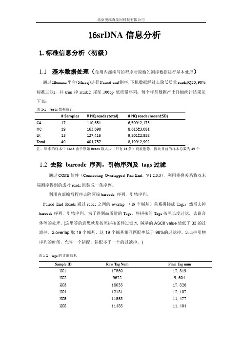
16srDNA信息分析1.标准信息分析(初级)1.1 基本数据处理(使用内部撰写的程序对原始的测序数据进行基本处理)通过Illumina平台(Miseq)进行Paired-end测序,下机数据经过去除低质量reads(Q20,90%标准过滤),并trim掉reads2 尾部100bp 低质量序列;每个样品数据产出详细统计结果见下表:表1-1 reads数据统计:CA17 110,651 6,509±2,175HC19 163,690 8,615±3,081LK13 127,416 9,801±2,858Total 49 401,757 8,199±2,992注:原来的样本中CA15由于原始Reads数太少(只有23条)而被删除,因此目前的样本总数为49个1.2去除barcode 序列,引物序列及tags过滤通过COPE软件(Connecting Overlapped Pair-End,V1.2.3.3),利用重叠关系将双末端测序得到的成对reads组装成一条序列。
利用内部编写程序去除两端barcode 序列,引物序列。
Paired End Reads通过reads之间的overlap (19个碱基)关系拼接成Tags;然后去掉barcode序列,引物序列。
为了得到高质量的Tags,将拼接的Tags按照长度过滤,去嵌合体等的处理。
(这里等的意思就是按照拼接条件过滤:1, 碱基的ASCII value值低于33的过滤掉。
2.overlap取19个碱基,这19个碱基相互匹配率低于98%的过滤掉。
3.去掉引物序列的时候,允许一个错配,错配多于一个的过滤掉。
)表1-2 tags的详细信息Sample ID Raw Tag Num Final T ag num HC1 17560 17,319HC2 9672 9,604HC3 18053 17,826HC4 12181 12,107HC5 11558 11,477HC8 11488 11,404HC9 16354 16,095HC10 21584 21,270HC11 7989 7926HC12 11561 11,449HC13 24909 24,660HC14 22979 22,736HC15 20747 20,549HC16 14857 14,728HC17 21171 21,002HC18 10700 10,605HC19 11359 11,247CA8 16203 16,040CA10 10925 10,560CA11 8254 7,690CA12 9479 9,053CA14 7947 7,584CA16 8221 8,093CA17 10666 10,479CA18 10787 10,651CA5 16344 16,154CA9 6047 5,861CA13 10290 10,1652高级信息分析2.1 OUT及其丰度分析2.1.1 OUT统计拼接的Tags经过优化后,在0.97相似度下利用qiime(v1.8.0)软件将其聚类为用于物种分类的OTU(Operational Taxonomic Units),统计各个样品每个OTU中的丰度信息,OTU的丰度初步说明了样品的物种丰富程度。
质谱分析软件操作规程

质谱分析软件操作规程质谱分析是一种常用的分析技术,可以用于物质的结构鉴定和组成分析。
在质谱分析中,使用质谱仪来将物质的分子或离子打散为离子,然后通过对离子的质量和相对丰度进行测量和分析,来得到物质的信息。
为了正确、高效地使用质谱分析软件,我们需要遵循以下操作规程:1. 软件的安装与启动:- 确保计算机符合软件的系统需求,进行软件的安装,并按照指引进行启动。
- 确保质谱仪与计算机的连接正常,并在软件中进行相关设置。
2. 仪器的校准与质量校验:- 在每次使用前,进行质谱仪的正常校准和质量校验,以确保测量结果的准确性和可靠性。
- 保持仪器的清洁和维护,定期进行保养和校准。
3. 样品的准备与运载:- 根据样品的性质和需要,选择适当的样品制备方法,并遵循相关的实验室操作规范进行准备。
- 将样品安装到质谱仪中,并设置相应的实验参数和扫描模式。
4. 数据的采集与分析:- 运行质谱仪,开始采集数据。
在数据采集过程中,可以对实验参数进行调整,以获取更准确和全面的数据。
- 将采集到的数据导入质谱分析软件中,进行数据处理和分析。
可以使用软件提供的工具和方法,对数据进行平滑、峰识别、峰面积计算等操作。
5. 结果的解释与报告:- 根据分析结果,解释样品的结构和组成,并进行研究或实验设计的讨论和推断。
- 根据需要,将结果整理成报告或文档,并保存记录。
在报告中,应包含详细的实验条件、数据处理方法和结果解释。
6. 实验的数据安全与保密:- 在进行实验和数据处理时,要遵循实验室的数据安全和保密规定,确保实验数据的完整性和保密性。
- 将数据备份和存储,以免数据丢失或损坏。
7. 实验数据的共享与交流:- 在保证数据安全和保密的前提下,可以与同事、合作者或上级进行数据共享和交流。
- 可以将数据导出为常见的数据格式,如Excel、PDF等,方便他人查看和分析。
8. 不断学习与提高:- 随着技术的发展和实验经验的积累,我们应不断学习和了解新的质谱分析方法和技术,提高质谱分析的能力和水平。
FAST科学数据说明文档说明书

FAST科学数据说明文档目录一、FAST简介 (2)二、数据类型说明 (2)三、数据终端参数设置说明 (3)一、FAST简介FAST的全称是“500米口径球面射电望远镜”,口径是500米。
实际观测的时候,变形为抛物面的区域的口径是300米,也就是说FAST的有效口径是300米。
计算灵敏度的时候需要用有效口径。
FAST观测的天顶角最大不超过40度,部分观测模式不能超过26.4度,超过范围会报规划错误。
1.1频段和接收机FAST目前有七套接收机。
现在一段时间使用的是19波束接收机,频率范围1.05GHz-1.45 GHz。
1.2观测模式目前已有的观测模式如下(括号中是代号,写观测计划文件时用):漂移扫描(Drift)带角度漂移(DriftWithAngle)跟踪(Tracking)带角度跟踪(TrackingWithAngle)运动中扫描(OnTheFlyMapping)多波束运动中扫描(MultiBeamOTF)源上-源外(OnOff)快照(SnapShot)多波束测试(MultiBeamCalibration)二、数据类型说明19波束接收机有脉冲星(psrfits)、谱线(sdfits)、baseband(dat)三种数据类型。
谱线终端数据根据选用数据记录方式分为两种,spec(F)—全带宽全分辨率,spec(W+N)—全带宽低分辨率+可选窄带高分辨率(可自行给定中心频率,默认为1420MHz)。
psr和spec数据终端可以选择记录全部19波束的数据,也可以只记录中心波束M01的数据。
baseband因受硬件方面的限制,目前只提供记录中心波束数据。
后端名称情况说明备注psr数据采样时间8.192*(acclen+1)us默认4K channels1K2K8K channels可选spec(F)500MHz,1M channels,频率分辨率:476.837158203125Hz 500M全带宽数据记录,只有以F 标识的FITS文件spec(W+N)500MHz+31.25MHz,64k channels,宽带频率分辨率:7.62939453125KHz窄带频率分辨率:476.837158203125Hz 宽带和窄带同时记录,窄带默认中心频率为1420MHz,也可自行指定。
pcoa分析

pcoa分析PCoA(Principal Coordinates Analysis,主坐标分析)是一种常用的多元统计分析方法,也被称为主坐标分解。
它是一种经典的降维技术,用于对多变量数据进行可视化和解释。
本文将介绍PCoA的基本原理、应用领域以及实际操作过程。
PCoA的基本原理是将高维空间中的数据映射到低维空间中,以便更好地进行数据观察和解释。
与其他降维技术相比,PCoA不需要对数据进行线性变换,因此更适用于非线性的数据。
它是一种基于距离矩阵的降维方法,通过计算样本间的距离来构造样本间的相似度矩阵,然后通过特征值分解来求解主坐标轴,最后根据主坐标轴的结果进行数据可视化和解释。
PCoA的应用领域非常广泛。
在生态学中,PCoA常用于分析多样性数据,帮助研究人员理解物种组成和生态系统的变化。
在遗传学中,PCoA用于分析基因频率的变化,以揭示不同种群之间的遗传关系和演化历史。
此外,PCoA还可以应用于社会科学、经济学、地理学等领域,帮助研究人员在多变量数据中发现模式和关系。
PCoA的实际操作过程如下。
首先,采集样本数据并计算样本间的距离。
距离可以是欧氏距离、曼哈顿距离、相关系数等多种形式。
其次,构建样本间的相似度矩阵,可以使用距离矩阵的逆作为相似度矩阵。
然后,对相似度矩阵进行特征值分解,求解主坐标轴。
最后,根据主坐标轴的结果进行数据可视化,可以使用散点图、气泡图等方式展示。
与其他降维技术相比,PCoA具有一些优点。
首先,PCoA能够保留数据的整体结构,不会造成太大的信息丢失。
其次,PCoA不依赖于线性假设,适用于非线性的数据分析。
此外,PCoA还具有较好的稳定性和可解释性,可以帮助研究人员理解数据之间的关系。
当然,PCoA也存在一些局限性。
首先,PCoA对异常值较为敏感,异常值的存在会对结果产生较大的影响。
其次,PCoA对数据的缺失值处理较为复杂,需要进行合适的插补或剔除。
另外,PCoA只能处理数值型数据,对于分类变量需要进行适当的编码转换。
16s分析之PCoA分析学习笔记
16s分析之PCoA分析学习笔记今天我们来一起学习一下PCoA分析:PCoA可以使用很多种距离的相异或者相似矩阵;基于关联矩阵,所以它也会有表征其重要性的特征根;############################################# ###################################################################### ##############导入我们需要的R包library("ggplot2")library("vegan")#找到我们需要的文件,mapping文件和beta多样性矩阵文件,现在我们先就bray_curtis做一个PCoAsetwd("E:/Shared_Folder/HG-QIIME-OTU")design =read.table("map_lxdjhg.txt", header=T, s= 1,sep="\t")setwd("E:/Shared_Folder/HG-QIIME-OTU/Beta")bray_curtis=read.table("bray_curtis_CSS_otu_table12072.txt",sep="\t",row.n ames= 1,header=T, s=F)#这里使用我们提前弄好的mapping文件和距离矩阵做一个匹配,主要就是两个文件处理编号检查一下,防止出现错误idx =rownames(design) %in% colnames(bray_curtis)#输出逻辑值idx#匹配上的筛选出来mappingsub_design =design[idx,]#初次作图,避免意外,展示一下,内心安稳sub_design#匹配上的矩阵筛出来,所以,做聚类矩阵的时候我们无所谓多少个处理,到时候,我们编一个mapping文件就可以了bray_curtis =bray_curtis[rownames(sub_design), rownames(sub_design)]#这里请记住pcoa函数,这里我们简单了解一下这个函数,第一个参数表示距离矩阵,第二个k代表选择多少个维度,在我们当然选择二维就够了,eig就是特征值,图片上常见的主成分得分就是使用这个值计算的pcoa =cmdscale(bray_curtis, k=2, eig=T) # k is dimension, 3 is recommended; eig iseigenvalues此时PCoA分析就算是做完了下一步就是出图的了:#提取我们作图需要的数据points =as.data.frame(pcoa$points) # 获得坐标点colnames(points)= c("x", "y") #坐标点命名eig = pcoa$eig#提取特征值为了计算坐标轴得分#将分组信息和我们的坐标轴合并points =cbind(points, sub_design[match(rownames(points), rownames(sub_design)), ])#我们是在做科研,显著性分析必然少不了#Adonis又称置换多元方差分析或非参数多元方差分析。
pcoa方法

pcoa方法
PCoA方法是一种常用的多元统计分析方法,全称为Principal Coordinate Analysis(主坐标分析),也被称为MDS(多维缩放)分析。
该方法主要用于研究样品间的相似性和差异性,通过将多维数据降维为二维或三维空间,将样品在空间中的位置表示出来,以便于观察和解释。
PCoA方法的基本思想是通过计算样品间的欧几里得距离或其他相似性指标,将多维数据降维为二维或三维空间,使得样品在空间中的距离尽可能地反映它们在多维空间中的相似性或差异性。
具体步骤如下:
1. 计算样品间的距离矩阵,可以使用欧几里得距离、Pearson相关系数、Bray-Curtis距离等多种相似性指标。
2. 对距离矩阵进行双中心化处理,即使得矩阵的行和列的和都为0。
3. 对双中心化后的距离矩阵进行特征值分解,得到特征值和特征向量。
4. 选择前k个最大的特征值对应的特征向量,将它们组成一个k维的特征空间。
5. 将每个样品在特征空间中的坐标表示出来,即可得到样品在二维或三维空间中的位置。
PCoA方法的优点是可以直观地展示样品间的相似性和差异性,同时可以用于多种类型的数据分析,如基因组学、微生物学、生态学等领域。
但是该方法也存在一些局限性,如对于高维数据的处理较为困难,对于非线性数据的处理效果较差等。
pcoa分析2篇

pcoa分析2篇pcoa分析是一种多元数据分析技术,可用于研究复杂的生物学、生态学和环境数据。
它可以将高维度的数据投影到二维或三维空间中,以便研究它们之间的差异和相似性。
本文将讨论什么是pcoa分析,如何进行pcoa分析以及该技术的潜在应用。
1. 什么是pcoa分析?pcoa分析,全称Principal Coordinates Analysis,是一种多元数据分析技术。
它是PCA(Principal Component Analysis)的扩展形式,可以用于研究多个特征的差异和相似性。
pcoa分析通过将高维度的数据降维到二维或三维空间中,以便更好地研究它们之间的相似性和差异性。
2. 如何进行pcoa分析?进行pcoa分析需要几个步骤:(1)准备数据集:将需要比较的样品的数据按照特征组成一个矩阵。
数据可以是基于多个特征的,也可以是基于一个特征的。
(2)计算样品间的距离矩阵:将数据矩阵转换为距离矩阵。
距离矩阵是样品之间的欧式距离或其他距离指标的矩阵。
(3)进行pcoa分析:将距离矩阵进行分析并绘制成二维或三维图形。
Pcoa分析可以使用多种软件包进行分析和绘图。
(4)解释结果:分析结果将给出每个样品的坐标值(即主坐标值)。
坐标值可以用来解释样品之间的差异和相似性。
3. pcoa分析的应用?pcoa分析是一种非常有用的多元数据分析技术。
它可以用于分析各种类型的生物和环境数据。
例如,研究环境因素(如温度、湿度、植被种类等)对生物群落的影响,可以使用pcoa分析来分析样品之间的相似性和差异性。
此外,pcoa分析也可以用于比较分类数据。
例如,在比较两个不同的物种群体时,可以将物种群体的适应性数据进行pcoa分析,以便比较它们的适应性。
总之,pcoa分析是一种强大的技术,可以用于研究各种类型的生物学和环境数据。
通过将高维度的数据降维到二维或三维空间中,可以更好地比较样品之间的相似性和差异性,从而帮助科学家更好地理解生物学,环境和生态学数据。
- 1、下载文档前请自行甄别文档内容的完整性,平台不提供额外的编辑、内容补充、找答案等附加服务。
- 2、"仅部分预览"的文档,不可在线预览部分如存在完整性等问题,可反馈申请退款(可完整预览的文档不适用该条件!)。
- 3、如文档侵犯您的权益,请联系客服反馈,我们会尽快为您处理(人工客服工作时间:9:00-18:30)。
Fast UniFrac is a new version of UniFrac that is specifically designed to handle very large datasets. Like UniFrac, Fast UniFrac provides a suite of tools for the com parison of m icrobial com m unities using phylogenetic inform ation. It takes as input a single phylogenetic tree that contains sequences derived from at least three different environm ental sam ples, a file m apping ids used in the tree to a set of unique sam ple ids (sam e form at as prior version 'environm ent file', and an (optional) category m apping file describing additional relationships between sam ples and subcategories for visualizations. For exam ple, in a given set of gut sam ples, you m ight define subcategories for different diets, different physical locations/dates, different species, and/or different treatm ents like antibiotics or high fat. For sam ple data click here. For citation, click here.Both the UniFrac distance m etric and the P test can be used to m ake com parisons. Both of these techniques bypass the need to choose operational taxonom ic units (OTUs) based on sequence divergence prior to analysis.Fast UniFrac allows you to:Determ ine if the sam ples in the input phylogenetic tree have significantly different m icrobial com m unities.Cluster sam ples to determ ine whether there are environm ental factors (such as tem perature, pH, or salinity) that group com m unities together.Determ ine whether system under study was sam pled sufficiently to support cluster nodes.Easily visualize the differences between sam ples graphically, with support for three dim ensional exploration of datasets and with m ultiple subcategory coloring.Please enter your em ail and password to continue. After you register you will be able to analyze up to 100000 unique sequences, up to 200sam ples, and perform significance test based on up to 1000 tree perm utations.If you wish to analyze m uch larger datasets than the defaults, please contact us and we will be happy to try to accom m odate you.Fast UniFrac tutorialIntroductionThis tutorial takes you through the steps of analyzing data in the Fast UniFrac web application. The purpose of this tutorial is to show you how to use the interface to find the im portant variables for describing phylogenetic variation am ong your sam ples: in this case, to test what types of physical or chem ical factors are m ost im portant for structuring bacterial diversity. The dataset used in this tutorial includes 50 of the 464 sam ples analyzed in Ley, RE, Lozupone, CA, Ham ady, M, Knight, R and JI Gordon. (2008). Worlds within worlds: evolution of the vertebrate gut m icrobiota. Nat. Rev. Microbiol. 6(10): 776-88 (Pubm ed). It includes sequences from 16S ribosom al RNA surveys of diverse freeliving bacterial assem blages and the guts of diverse m am m als and term ites. At the end of this tutorial, you should be fully equipped to test hypotheses about your own sequences.Also included in this tutorial are other exam ple files you m ay use to explore som e of the other features of Fast UniFrac.Example data filesTo use Fast UniFrac, you need three files: a tree file, a sam ple id m apping file, and a category m apping file. The tree file contains a phylogenetic tree, in Newick form at. The sam ple id m apping file contains a table showing how m any tim es each taxon (from the tree) occurred in each of your sam ples. The category m apping file contains additional m etadata about the sam ples, and is a table relating each sam ple to param eters you have m easured such as tem perature, pH, etc. In general, people usually prepare the two m apping files using Excel, although it is im portant to save them as plain text form at and not as Excel docum ents.You can either generate your own tree file, or use one of the reference trees. The PhyloChip reference tree m atches the probes on the PhyloChip and is useful for analyzing PhyloChip data; the Greengenes reference tree is from the Greengenes core set and is a phylogenetically diverse and representative set of bacteria. These trees are built using 16S rRNA, although you can use trees built from any m olecule, not just the 16S, or even trees constructed from m orphological or other data.The sam ple id m apping file m ust be generated m apping the sequence ids in the tree file with the sam ple ids used in your study. In other words, exactly the sam e taxon nam es m ust be used in your tree and in your sam ple id m apping file.The category m apping file m aps your sam ple ids to additional m etadata, such as subcategories, and sam ple descriptions. This file can be autogenerated but it is highly recom m ended that you generate one that is m eaningful for the variation you plan to exam ine in your studies. For exam ple, if you were studying the effects of diet on the gut com m unities of conventional and hum anized m ice, you m ight want one colum n indicating whether the sam ple was from a conventional or a hum anized m ouse, another colum n indicating whether the m ouse was on a chow diet or a high-fat diet, another colum n containing the com bination of these two colum ns (i.e. diet and hum anized/conventional), etc.In this section, several exam ple files are listed, not all of which are used in this tutorial.Greengenes coreset reference datasetsThis is the tree and the sequences m atching the Greengenes core set as of May 2009. These files are useful for m apping your sequences against known bacterial diversity.1. Greengenes coreset tree (May 09)2. Greengenes coreset fasta (May 09)NRM data (demo subset)These data are from the Ley et al. 2008 Nature Reviews Microbiology paper referenced above, and provide an exam ple of m apping heterogeneous reads to the Greengenes core set tree so that the com m unities can be com pared by UniFrac. The sam ple ID m apping file was generated by blasting the dataset from the paper against the Greengenes_coreset_fasta file linked above, and the category m apping file was constructed m anually to provide a range of fine- and coarse-grained representations of the environm ental data.1. Ley et al exam ple sam ple ID m apping file2. Ley et al exam ple category m apping fileExample PhyloChip dataExam ple data from Sagaram et al. 2009 AEM paper (Pubm ed) for use with PhyloChip reference tree.1. Sagaram et al PhyloChip sam ple ID m apping file2. Sagaram et al PhyloChip category m apping fileCrump et al dataThese sequences are from Crum p et al. 1999 "Phylogenetic analysis of particle-attached and free-living bacterial com m unities in the Colum bia river, its estuary, and the adjacent coastal ocean", AEM 65:3192 (Pubm ed). This dataset was used in the original online UniFrac tutorial (Pubm ed)so are provided again here with two im portant changes. We provide an exam ple category m apping file that contains additional m etadata about each of the sam ples.1. Crum p et al exam ple tree file2. Crum p et al exam ple sam ple ID m apping file3. Crum p et al exam ple category m apping fileMegablast protocol and sample mapping generation scriptThe application of UniFrac to large sequence sets, such as those generated with pyrosequencing, is also lim ited by the com putational power needed to m ake a de novo phylogenetic tree using standard m ethods, such as neighbor joining, likelihood, or parsim ony m ethods. In order to prepare phylogenetic trees for input into UniFrac from very large datasets, we recom m end using QIIME. The best source for inform ation about QIIME are the website and the QIIME paper, which you can get at the following links:1. Source code2. QIIME allows analysis of high-throughput com m unity sequencing dataThe quickest way to get started with QIIME is using the virtual m achine.One potential workflow for working with ñarge datasets is to use QIIME to:1. Preprocess sequences to handle low quality reads2. Select OTUs3. Generate a phylogenetic tree , and then use the QIIME script convert_otu_table_to_unifrac_sam ple_m apping.py, to generate the proper input files forthe Fast UniFrac web interface.In the initial release of Fast UniFrac, we also described the following procedure for generating a phylogenetic tree, which is based on m apping sequences to their closest relative in a reference tree using BLAST. This functionality is now in QIIME, and we recom m end using QIIME for this step, but retain this docum entation below for those who m ay still be interested in using itThe BLAST to greengenes protocolWe illustrate that the analysis of such large sequence sets can be carried out by assigning them to their closest relative in a phylogeny of the Greengenes core set (DeSantis et al., 2006) using BLAST’s m egablast protocol (Altschul et al., 1990). Below is a detailed protocol for carrying out this analysis. Note thata different BLAST database can be substituted for use with any reference tree.1. Create the Greengenes BLAST database:This link is a fasta file containing the sequences from the greengenes coreset. This fasta record can be form atted into a BLAST database using the com m and:f o r m a t d b-i G r e e n G e n e s C o r e-M a y09.r e f.f n a-p F-o F-ng g_c o r e s e t2. Perform the megablast search:A fasta record of your sam ples can be BLASTed against the gg_coreset BLAST database created in step 1 using the following com m and:b l a s t a l l-p b l a s t n-n T-d g g_c o r e s e t-i-e1e-30-b5-m9-o b l a s t_o u t p u t.t x tNote that the -m 9 flag is essential because it specifies the hit table output form at that the script below requires.Also note that the sequence nam es m ust conform to the following form at:s a m p l e N a m e D e l i m i t e r s e q u e n c e I dFor instance, if you sequenced 2 clones from each of two sam ples nam ed SA and SB, valid sequence nam es m ight be:S A#01S A#02S B#01S B#02If you have not nam es the sequences according to this convention, it is possible to also use a m apping file describing which sequence is from which sam ple. See docum entation within the code for m ore details on this.3. Use this python script and the BLAST output from step 2 to create an environment file that can be used with UniFrac:Note that the PyCogent toolkit m ust be downloaded from SourceForge and the cogent directory should be on your PYTHONPATH.You can then use the code as follows:p y t h o n c r e a t e_u n i f r a c_e n v_f i l e_B L A S T.p y<b l a s t_o u t p u t.t x t><o u t f i l e_p a t h.t x t><s a m p l e_n a m e_d e l i m i t e r>blast_output.txt: Path to the hit tables from the BLAST searchesoutfile_path.txt: Path to where the environm ent file will be savedsam ple_nam e_delim iter: A delim iter (e.g. a #) that separates the sam ple nam e from the sequence id.Steps1. Create a phylogenetic tree containing sequences from samples that you would like to compare, or select a reference tree.The tree should be rooted, and m ust have branch lengths to use Fast UniFrac. Typically, the tree is rooted by including an outgroup, e.g. an archaeal sequence to root the bacteria, but we som etim es use m idpoint rooting as well. If an unrooted tree is supplied, UniFrac will assign a root arbitrarily. If you have extra sequences in the tree that are not annotated by sam ple, they will autom atically be rem oved from the tree when you upload the file, so the outgroup will not be included in the analysis. If no sequences appear in the tree after upload, the m ost likely problem is that there was an issue with your sam ple ID m apping file (for exam ple, you m ight have used GenBank identifiers in the tree, but NCBI GIs in the sam ple ID m apping file, which wouldn't m atch each other).There are m any different program s that you can use for sequence alignm ent and/or the phylogeny include the NAST alignm ent tool, PyNAST, FastTree, ARB, ClustalW, MUSCLE, PHYLIP, PAUP, or MrBayes. For 16S rRNA sequences, we prefer PyNAST for alignm ent. For generating trees from large dataset, we prefer FastTree for de novo tree generation trees or m apping sequences to their closest relative in a reference tree. These preferred options as well as several others can be run using QIIME. For large datasets, it is greatly preferred to select OTUs prior to the alignm ent and tree building step. This cuts down on the com putation tim e and does not have an effect on the results. Because UniFrac depends on branch lengths, it is im portant to look at your tree to ensure that you don't see long branches that result from m isalignm ent rather than from long periods of evolution. At the end of this process, you can export the tree in Newick form at for upload into the UniFrac interface.Alternatively, you can choose one of the reference trees provided and m ap your sequences to this tree. This can be useful, particularly for large datasets, such as those produced by 454 pyrosequencing, since creating a single phylogenetic tree with all sequences m ay not be feasible with the program s listed above. One sim ple way to m ap your sequences onto their closest relatives in a reference tree is use m egablast. In this tutorial, the original sequences from the NRM paper were assigned to their closest hit in the 11-Aug_2007 version of the greengenes coreset (can be downloaded from /Download/Sequence_Data/Fasta_data_files/). Sequences with no hit or that m atch with an e-value greater than e-50 were dropped from this exam ple dataset.For the purpose of this tutorial, we provide the greengenes coreset tree in Newick form at that we exported from an arb database that is available for download at /Download/Sequence_Data/Arb_databases/greengenes236469.arb.gz. A sm all num ber of sequences were added to this tree using parsim ony insertion in arb so that the fasta data files and tree for the core set were in sync. The resulting tree (Greengenes coreset tree (May 09)) and corresponding sequences (Greengenes coreset fasta (May 09)) can downloaded, but please note that this tree can be im ported to your history and does not need to be re-uploaded. In order to im port the GreenGenes reference tree to your history follow these steps:1. In the upper m enu, go to Shared Data - Data Libraries:2. Then, select 'GreenGenes coreset tree (May 09):3. Click on the checkbox next to 'GreenGenesCore-May09.ref.tre' and, finally, on the 'Go' button:4. The reference tree is now in your history and you can use it.2. Create a sample ID mapping file.This file m aps each sequence ID in the tree to the sam ple ID that it cam e from. This m ust be done m anually (or via a script): for each sequence, type the sequence ID used in the tree, then a tab, then the sam ple ID that it com es from, then optionally, another tab and then the num ber of tim es each sequence was observed (sequence abundance).The sequence abundance colum n is im portant if you have dereplicated the sequence data in any way (e.g. choosing OTUs and only including a representative sequence in the tree, rem oving exact duplicate sequences, or pre-screening clones using RFLP patterns prior to sequencing), and you are planning on using tools in the interface that consider differences in relative abundance (e.g. weighted UniFrac). It is fine to use a tree and sam ple ID m apping file with all of the sequences (e.g. 5 duplicate sequences in the tree each with a weight of 1 rather than 1 representative sequence with a weight of 5) and to perform abundance-based analyses, although dereplicating the data will allow you to process larger datasets.For PCoA analysis, it is m ost convenient to nam e each environm ent so that sam ples of the sam e type have nam es that start with the sam e first 1, 3, or 5 letters or that have sam ple types followed by a period, hash, or plus character (this allows you to apply colors in the PCoA scatterplots later).In this exam ple, there are 50 bacterial sam ples from the following sam ple types: Surface and subsurface saline water (Sws, and Swb respectively), Nonsaline water (Nw), Saline sedim ents (Sse), Nonsaline sedim ents (Nsa), Soils (Nso), the Vertebrate gut (Vg) and the Term ite gut (Tg). We'll label each sam ple with its 2-3 letter sam ple code, followed by a hash, and a unique num ber because our hypothesis is that the organism s from the sam e overall environm ent should be m ore sim ilar to one another.The following is a short snippet of a sam ple ID m apping file. The first colum n is the sequence ID, the second colum n is sam ple ID, and the last colum n is the num ber of tim es the sequence was observed.150394T g#12491150394T g#12512215260N s o#651215260N s o#129416073V g#h#111...For the purpose of this tutorial, we provide a sam ple ID m apping file called fastunifrac_Ley_et_al_NRM_2_sam ple_id_m ap.txt.zip sam ple ID m apping file.3.Create a category mapping file.The category m apping file relates sam ple nam es in the sam ple ID m apping file to their related m eta data (defined via subcategory colum ns) and descriptions of where the sam ples cam e from. The descriptions can be accessed throughout the results interface in order to m ake them easier to interpret. The subcategory colum ns allow for dynam ic coloring of PCoA results in the 3d viewer to determ ine which categories are related to which principal coordinate axes.For the purpose of this tutorial, we provide a category m apping file called Ley et al exam ple category m apping file with 4 subcategory colum ns that define for each sam ple (1) which sam ple type it is from(EnvType), (2) whether the sam ple cam e from a freeliving bacterial assem blage or from the gut (FreelivingGut), (3) whether the freeliving com m unities were saline or nonsaline (SalineNon), and whether they were from aquatic (Water) or "Particulate" sam ples such as soils and sedim ents (WaterPartic). There is also a short description of each sam ple in the final colum n.The file form at is tab-delim ited text. The first line is a header line that m ust start with a "#" character.Optionally, a general description of the input files can be included in the lines im m ediately following the header line that start with a "#". This description will be included in the upload and results screens so that relevant inform ation can be easily accessed.The first colum n m ust be nam ed Sam pleID, m ust contain unique (short, m eaningful) sam ple IDs containing only alphanum eric characters. (With the exception of ".", "+", and "#" characters.)The second colum n to "n-1 th" colum n are subcategories. These can be anything (random assignm ent if you want) but each subcategory should a sm all num ber of distinct values <= num ber of sam ples. There m ust be at least two unique values for each category.The last colum n m ust be nam ed "Description" and contains the short descriptions for the sam ples.#S a m p l e I D E n v T y p e F r e e l i v i n g G u t...D e s c r i p t i o n#G e n e r a l d e s c r i p t i o n o f a n a l y s i s l i n e1(o p t i o n a l)#G e n e r a l d e s c r i p t i o n o f a n a l y s i s l i n e2(o p t i o n a l)#...T g#1249T e r m i t e G u t G u t...W h o l e g u t o f t h e w o o d-f e e d i n g t e r m i t eT g#1251T e r m i t e G u t G u t...W h o l e g u t o f t h e f u n g u s-g r o w i n g t e r m i t e M a c r o t e r m e s g i l v u sN s o#65S o i l F r e e l i v i n g...U n c u l t i v a t e d a g r i c u l t u r a l s o i l i n W i s c o n s i nN s o#1209S o i l F r e e l i v i n g...S o i l f r o m a f e r t i l i z e d S w i t z e r l a n d p l o t i n t h e D O K.V g#h#111V e r t e b r a t e G u t G u t...F e c e s f r o m A n g o l a n C o l o b u s M o n k e y f r o m t h e S t L o u i s Z o o....For the purpose of this tutorial, we provide a category m apping file called fastunifrac_Ley_et_al_NRM_3_category_m ap.txt.zip sam ple ID m apping file.4. Go to the Fast UniFrac web site.If you're reading this tutorial, you already know how to get here. You will need to register and log in to com plete the tutorial, because we restrict the num ber of sequences that unregistered users can analyze. The reason for this is that m any of the analyses are com putationally expensive, so we need to keep track of which groups are using a lot of resources to ensure fair access for everyone. Please note that if you have previously registered for the original UniFrac interface, you will have to contact m icrobiom ehelp@ to register for FastUniFrac. We apologize for this inconvenience.5. The Fast UniFrac upload screenAfter you have logged in, you have to upload your sam ple ID m apping file and your category m apping file. To get to the upload page, click 'Get data' on the Tools panel and then 'Upload file':Then, the upload page will appear:First, upload your sam ple ID m apping file. Click 'Browse' below where it says File, and navigate to your sam ple ID m apping file (in this case, fastunifrac_Ley_et_al_NRM_2_sample_id_map.txt). One com m on problem is that you m ight have your sam ple ID m apping file saved as a Word docum ent: this will NOT work, because Word uses a proprietary file form at that is difficult for other program s to read. If you are saving your sam ple ID m apping file from Word, rem em ber to save it as Plain Text, NOT as Microsoft Word. If you are using Excel, save as Tab-delim ited Text. At the end of thisprocess, your screen should look like this:state - blue color) will appear in the history panel:While the sam ple ID m apping is uploading, you can start with the category m apping file upload. In order to upload your category m apping file follow the above steps, but now navigate to your category m apping file (in this case, fastunifrac_Ley_et_al_NRM_3_category_map.txt). This file is m ost easily created in Excel, rem em ber to save as Tab-delim ited text.If you have your own tree file, you can upload it following these sam e steps. In this tutorial, we will use the 'GreenGenes Core - May 2009' tree, which is already on the system.Once all the files are uploaded (the datasets in the history panel are in green color) you can start any of the available analysis in Fast UniFrac.6. Measuring the overall difference between each pair of samples.In order to generate the raw distances between each pair of sam ples using the UniFrac m etric, first choose the Sample Distance Matrix option from the Tool panel, under the 'Fast UniFrac' section.On the Sam ple Distance Matrix page you can select the reference tree, sam ple ID m apping file and the category m apping file you want to use to perform the analysis. First, select the 'GreenGenes Core - May 2009' tree using the drop-down m enu below 'Select reference tree'. Next, select the '1: fastunifrac_Ley_et_al_NRM_2_sam ple_id_m ap.txt' file and the '2: fastunifrac_Ley_et_al_NRM_3_category_m ap.txt' file using the drop-down m enus below 'Select sam ple ID m apping file' and 'Select category m apping file', respectively. If you then click the 'Execute' button, you will get a m essage saying that your job has been subm itted to the queue, and two new datasets will appear in the History panel. When the datasets are green (tim e depending on server load) you can view them clicking on the eye icon. The first dataset will display a screen like the following. containing the distance m atrix that relates each pair of environm ents:Moving your m ouse over the m atrix cells will display the raw score for that pair of sam ples and the sam ple description, to help you to m ore easily interpret the data.At the bottom of the m atrix, you will see a color key and a link to download the im age.This distance m atrix is colored by quartile: the sm allest distances (m ost sim ilar pairs) are colored blue, and the largest distances (m ost different pairs) are colored gray. In this exam ple, all of the distances are fairly sim ilar (num erical values ranging from0.68 to 0.86), indicating that any given pair of environm ents shares less than one third, and as little as 15%, of the total phylogenetic diversity contained by both together. However, the distance m atrix by itself is often difficult to interpret: the pattern of sim ilarities is not very clear.The second dataset that appears in the History panel is a tab-delim ited file with the raw distance m atrix. You can download it by clicking on the disk icon.7. Clustering the samples.It can be useful to see how the environm ents cluster together since there are often patterns in the clustering that could not have been determ ined from the pattern of significant differences alone.Select the Cluster Samples option from the Tool panel, choose the reference tree, sam ple ID m apping and category m apping files following the stepsdescribed above and then click the 'Execute' button.As in the Distance Matrix case, this analysis also generates two new datasets in the History panel. The result is a tree relating the different environm ental sam ples. The first dataset is a graphic representation of the tree and the second one is the tree in Newick form at, so you can use it in other program s such as TreeView.In the graphic representation of the tree, if you m ove your m ouse over each sam ple ID, it will display the sam ple description, helping you m ore easily interpret the clustering patterns of your sam ples.In this case it is easy to see that the different sam ple types cluster together: for exam ple, the term ite gut sequences (Tg) form a cluster at the upper part of the plot, below them all the vertebrate gut sequences (Vg) are a clum p, etc.This figure shows the power of UniFrac: although m any sam ples are not significantly different from one another when corrected for m ultiple com parisons, biologically interesting patterns still com e out of the analysis.However, to be confident that the results are correct, it is necessary to perform the Jackknife Sample Clusters analysis, which will sam ple a sm aller num ber of sequences from each environm ent and tell you whether the clusters are well-supported.When we perform this analysis with default param eters, the nodes are colored like this:This m eans that if 37 sequences are chosen from each sam ple (the m axim um am ount that can be resam pled without dropping the sm allest sam ple from the analysis), the best nodes are recovered between 79% and 96% of the tim e (colored green and yellow respectively), which m eans that the support for them is relatively strong.If instead we increase the num ber of sequences required per sam ple (by changing the Minim um sequences to keep on the Jackknife Sam ple Clusters page), som e of the sam ples will be discarded, and the support for the rem aining clusters m ay change.The m ost reasonable value to use for Minim um sequences to keep is about 75% of the sm allest sam ple you want to include in the analysis, but in practice people usually just use the sm allest sam ple (despite the fact that there is then no resam pling perform ed on that sam ple).8. Perform Principal Coordinates Analysis (PCoA).The cluster diagram s are useful for showing which environm ents are m ost closely related to one another, but it is also im portant to see if the environm ents are distributed along any axes of variation that can be interpreted easily (e.g. a pH or tem perature gradient).Select the PCoA option from the tool panel, choose the reference tree, sam ple ID m apping and category m apping files following the steps described aboveand then click the 'Execute' button.form ats of the PCoA analysis:。