R语言偏最小二乘法判别分析(pls-da)
细胞代谢组学研究及应用进展

细胞代谢组学研究及应用进展【关键词】细胞代谢组学;研究方法与应用;综述【摘要】细胞代谢组学作为代谢组学研究的一个新兴的方向,在病原体感染、肿瘤研究、药物作用机制及药物研发、毒性评价等多个领域都有所应用。
可解决基本的生物学问题,并允许观察细胞内的代谢现象。
现简要综述细胞代谢组学的主要研究方法及其应用方面的研究进展。
1.细胞代谢组学的研究方法细胞代谢组学实验一般可分为几个步骤:细胞增生培养或刺激、淬灭、代谢物提取、样品检测和数据处理。
1.1细胞淬灭细胞淬灭是指快速使细胞内的酶失活,阻止代谢物变化。
理想的淬灭技术应在不损害细胞、不造成细胞内代谢物泄漏的前提下确保胞内酶迅速失活。
Hounoum等考察3种细胞淬灭方式对NSC-34鼠神经元细胞的影响,分别为-40℃甲醇淬灭、-20℃甲醇淬灭及迅速冻存于-80℃后加入4℃甲醇淬灭。
实验结果显示-40℃甲醇是用于该细胞最为理想的淬灭方式;有研究发现甲醇会破坏细胞膜结构,从而导致无法控制的细胞内代谢物泄漏,故常在甲醇中加入缓冲液如HEPES及AMBIC以维持离子强度,避免渗透冲击。
而对于贴壁细胞,液氮冷冻被是停止其酶活性的最佳方法,Zhao等比较了液氮和75%甲醇(-80℃)2种溶液对副溶血性弧菌细胞的淬灭效果,结果发现75%甲醇(-80℃)淬灭时,细胞发生代谢物泄漏;液氮淬灭速度快,且不存在代谢物泄漏问题。
1.2代谢物提取代谢物具有不同的化学和物理性质,如大小、质量、极性、溶解性等,而细胞代谢组学要求找到一种合适的提取方式,尽可能多地把胞内所有代谢物定量提取出来。
因此,提取方法应该有效而没有选择性和破坏性。
提取过程应有效地从细胞中释放代谢物,避免潜在干扰,确保最小代谢物损失。
胞内代谢物通常单独用有机溶剂,或与水结合,或与其他有机溶剂结合,在不同温度条件下提取。
经典的酸性和碱性提取剂也可分别用来提取对酸、碱稳定的化合物。
对于悬浮细胞,常用含水甲醇、含水乙腈或纯甲。
r语言最小二乘法
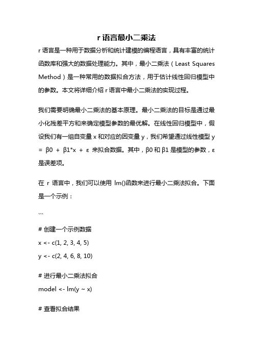
r语言最小二乘法r语言是一种用于数据分析和统计建模的编程语言,具有丰富的统计函数库和强大的数据处理能力。
其中,最小二乘法(Least Squares Method)是一种常用的数据拟合方法,用于估计线性回归模型中的参数。
本文将详细介绍r语言中最小二乘法的实现过程。
我们需要明确最小二乘法的基本原理。
最小二乘法的目标是通过最小化残差平方和来确定模型参数的最优解。
在线性回归模型中,假设我们有一组自变量x和对应的因变量y,我们希望通过线性模型y = β0 + β1*x + ε 来拟合数据。
其中,β0和β1是模型的参数,ε是误差项。
在r语言中,我们可以使用lm()函数来进行最小二乘法拟合。
下面是一个示例:```# 创建一个示例数据x <- c(1, 2, 3, 4, 5)y <- c(2, 4, 6, 8, 10)# 进行最小二乘法拟合model <- lm(y ~ x)# 查看拟合结果summary(model)```上述代码首先创建了一个示例数据,其中x是自变量,y是因变量。
然后,通过lm()函数进行最小二乘法拟合,将结果保存在model 对象中。
最后,使用summary()函数查看拟合结果。
在输出的结果中,我们可以得到拟合的回归方程的系数估计值、残差平方和、决定系数等信息。
例如,拟合结果中的Coefficients一节显示了回归方程的系数估计值,其中Intercept对应β0,x对应β1。
除了lm()函数,r语言还提供了一些其他函数用于进行最小二乘法拟合,例如lsfit()函数和nls()函数。
lsfit()函数适用于一般的线性回归模型,而nls()函数适用于非线性回归模型。
这些函数的使用方法可以参考官方文档或相关教程。
最小二乘法不仅适用于线性回归模型,还可以用于其他类型的统计建模,例如多项式回归、逻辑回归等。
对于这些模型,r语言同样提供了相应的函数进行拟合。
除了最小二乘法,r语言还提供了其他的统计建模方法,例如广义线性模型(Generalized Linear Model)、岭回归(Ridge Regression)等。
偏最小二乘法

偏最小二乘法 ( PLS)是光谱多元定量校正最常用的一种方法 , 已被广泛应用 于近红外 、 红外 、拉曼 、核磁和质谱等波谱定量模型的建立 , 几乎成为光谱分析中建立线性定量校正模型的通用方法 〔1, 2〕 。
近年来 , 随着 PLS 方法在光谱分析尤其是分子光谱如近红外 、 红外和拉曼中应用 的深入开展 , PLS 方法还被用来解决模式识别 、定量校正模型适用性判断以及异常样本检测等定性分析问题 。
由于 PLS 方法同时从光谱阵和浓度阵中提取载荷和得分 , 克服主成分分析 ( PCA)方法没有利用浓度阵的缺点 , 可有效降维 , 并消除光谱间可能存在的复共线关系 , 因此取得令人非常满意的定性分析结果 〔3 ~ 5〕 。
本文主要介绍PLS 方法在光谱定性分析方面的原理及应用 实例 。
偏最小二乘方法(PLS-Partial Least Squares))是近年来发展起来的一种新的多元统计分析法, 现已成功地应用于分析化学, 如紫外光谱、气相色谱和电分析化学等等。
该种方法,在化合物结构-活性/性质相关性研究中是一种非常有用的手段。
如美国Tripos 公司用于化合物三维构效关系研究的CoMFA (Comparative Molecular Field Analysis)方法, 其中,数据统计处理部分主要是PLS 。
在PLS 方法中用的是替潜变量,其数学基础是主成分分析。
替潜变量的个数一般少于原自变量的个数,所以PLS 特别适用于自变量的个数多于试样个数的情况。
在此种情况下,亦可运用主成分回归方法,但不能够运用一般的多元回归分析,因为一般多元回归分析要求试样的个数必须多于自变量的个数。
§§ 6.3.1 基本原理6.3 偏最小二乘(PLS )为了叙述上的方便,我们首先引进“因子”的概念。
一个因子为原来变量的线性组合,所以矩阵的某一主成分即为一因子,而某矩阵的诸主成分是彼此相互正交的,但因子不一定,因为一因子可由某一成分经坐标旋转而得。
pls (partial least squares analysis):pls(偏最小二乘法)
---------------------------------------------------------------最新资料推荐------------------------------------------------------pls (partial least squares analysis):pls(偏最小二乘法)PLS (PARTIAL LEAST SQUARES ANALYSIS) Introduction Partial Least Squares (PLS) Analysis was first developed in the late 60s by Herman Wold, and works on the assumption that the focus of analysis is on which aspects of the signal in one matrix are related directly to signals in another matrix. It has been developed extensively in chemometrics, and has recently been applied to neuroimaging data. In the application to imaging data, it has been used to identify task-dependent changes in activity, changes in the relations between brain and behaviour, and to examine functional connectivity of one or more brain regions. PLS has similarities to Canonical Correlation in its general configuration, but is much more flexible. This GUI is the first major release of PLS for neuroimaging. It has been in development for some time, and although this version appears stable, there are always things that can be improved. We are also planning several enhancements, such as univariate testing of means and correlations, advanced plotting routines and higher-order analyses. Please check our website regularly to see if there are updates. PLS computes a matrix that defines1/ 11the relation between two (or more) matrices and then analyzes that cross-block matrix. In the case of TaskPLS, the covariance between the image dataset and a set of design contrasts can be calculated (an equivalent procedure is described below). The covariance images are analyzed with Singular Value Decomposition (SVD) to identify a new set of covariance images that correspond to the strongest effects in the data. For BehaviourPLS, task-specific correlations of brain activity and behaviour are computed (across subjects), combined into a single matrix, which is then decomposed with SVD. The resultant patterns identify similarities and differences in brain-behaviour relations. Creating Datamat Regardless of which type of PLS is to be conducted, the data must be in a form such that all data for all subjects and tasks that are to be analyzed are contained in a single matrix. For image data in general, it is assumed images have been standardized in some manner so that they are all the same shape and size. For PET and MRI data, PLS works best if you use the smallest smoothing filter possible (e.g., no more than twice the voxel size). For ERP data, any filtering, or replacing data in bad channels, etc. must also be done before creating the PLS data matrix. The Session Profile part of our program loads brain images or ERP---------------------------------------------------------------最新资料推荐------------------------------------------------------ waveforms, strings each one out into a vector and then stacks the vectors one on top of the other to make the large data matrix (called datamat in the PLS programs). Each image (also called subject data file) represents one subject under one condition. For brain images, the script also eliminates voxels that are zero or non-brain using a threshold, which is specific to each type of image data. Removing the zero and non-brain voxels reduces the size of the datamat considerably and streamlines the computations. Unfortunately, this can restrict the data set if image slices were not prescribed in the same way for all subjects. To make life easy, a mask is created based on the voxels that are common for all subjects. After the datamat is re duced, a vector (‘coords’) is generated to remap the reduced datamat into image space again. PET Images: The code is written assuming you used the SPM99 sterotaxic template with 4x4x4 mm voxels, which creates images having 34 slices each with 40 voxels in the X and 48 voxels in the Y dimensions. For PET scans, the threshold to define brain voxels is 1/4 of the maximum value for a particular subject. The final datamat will have S by C rows and V columns (where S is the number of subjects and C is the number of scans or conditions, V is the number of3/ 11common brain voxels in the image data set). ERP: For ERP data, all channels of a subject data file are strung out into a single vector and the vectors are then stacked one on top of the other. The datamat will have S by C rows and E by T columns (where S is the number of subjects, C is the number of conditions, E is the number of channels, and T is the number of time points in the subject data file). If, after creating the datamat, it becomes clear that a particular set of ERP channels is bad for most of the subjects, those channels can be eliminated from the analysis using the GUI. As well, single subject data can also be eliminated from the analysis using the GUI. fMRI: Creating the datamat for fMRI datasets combines the two approaches above. This allows you to run the analysis either on each subject or as a group. Common voxels across subjects and/or runs are identified, then a single row vector is created for each subject, separately for each condition. The datamat will be S by C rows and V by T columns (where S is the number of subjects, C is the number of conditions, V is the number of common voxels, and T is the number of images defined by the user to account for the lag in the hemodynamic response). TaskPLS: Analysis using Grand Mean Deviation The TaskPLS is designed to identify whole-brain (scalp) patterns of activity that---------------------------------------------------------------最新资料推荐------------------------------------------------------ distinguish tasks. In TaskPLS, a pattern may represent a combination of anticipated effects and some unanticipated ones. The Grand Mean Deviation analysis is based on representing task means as the deviation around the grand mean computed for each voxel and/or time point. The data are thus averaged within a task, leaving out the within-task variability. (We are exploring the possibility of a constrained PLS solution, where a set of apriori contrasts are used to define the solution space). Next the SVD algorithm is used to get the following three components: brainlv (or salience), singular value (s), and designlv (salience for design). The design scores and brain scores (or scalp scores in ERP) are obtained from the formula below: design scores LV(n) = designlv brain scores LV(n) = datamat * brainlv The saliences for design (designlv) and brain (brainlv) are orthonormal, or standardized. To make comparisons across latent variables easier to visualize, we compute unstandardized saliences. This is accomplished by weighting the saliences by their singular values for the latent variable. All eigenimages and ERP salience plots use the unstandardized saliences. TaskPLS is run by clicking the Run PLS Analysis button. All results are saved into a specified file.5/ 11The results will include all data mentioned above, and other useful information. The TaskPLS results can be displayed by clicking the Show PLS Result button in the main GUI window. For PET and Blocked fMRI, the saliences (eigenimages) and bootstrap ratio images are displayed in a montage that includes all the slices for the LV. For Event-Related fMRI, the results are displayed in a montage as follows: each row represents one lag point, thus the number of rows equals the specified temporal window; each column represents the slices in the image. For ERPs, the LV saliences are displayed as a scalp plot, including only the selected electrodes and epoch. In the results window, you will also find options to display: scatterplots of brain (scalp) scores with design scores, designLV bar plots, and bar plots of the singular values and permutation test results. Behaviour PLS: Analysis using Behaviour Data The BehaviourPLS first calculates a correlation vector of behaviour and brain within each task, then stacks these vectors into a single matrix that is decomposed with SVD. Behaviour PLS has the potential to identify commonalities and differences among tasks in brain-behaviour relations. The behaviour matrix contains one or more behavioural measures that are thought to relate to the measured brain activity. The number of rows in the behaviour---------------------------------------------------------------最新资料推荐------------------------------------------------------ matrix and datamat should be the same, with a separate columnfor each behavioural measure. Since this matrix is created outside of the GUI, it is important that the order of subjects and conditions be identical to the order defined using the GUIto create the datamat. As for the TaskPLS, the results window initially contains plots of the unstandardized saliences. Within the results window, you can also display scatterplotsof brain (scalp) scores with behaviour, bar plots showing the magnitude of the brain-behaviour correlation with confidence intervals, and bar plots of the singular values and permutation test results. In the brain (scalp) scores by behaviour plots, the linear fit is also plotted to better view the scatter around the correlation. Tests of Significance PERMUTATION TEST: The significance of the latent variable, as a whole, is assessed using permutation tests. We assess the magnitude of the singular values by asking the question: With any other random set of data, how often is the value for s as large as the one obtained originally? To generate this answer, subjects are randomly reassigned (without replacement) to different conditions, and the PLS is recalculated. Orthogonal procrustes rotation is applied to the resulting BehavLV or7/ 11DesignLV to correct for reflections and rotations of the resampled data, and the singular values are recalculated based on this rotation (Milan and Whittaker 1995). If the probability of obtaining higher singular values is low, the latent variable is considered to be significant. For both task and behaviour, 500 permutations are generally sufficient, although probability estimates are typically stable at about 100 permutations. BOOTSTRAP: Bootstrap estimation is used to assess the reliability of the brain saliences. In this case, subjects are resampled with replacement. A new datamat, and for BehaviourPLS, a new behaviour matrix are created, and the PLS is recalculated. Thus, unlike for the permutation test, the assignment of subjects to conditions is maintained, but the subjects contributing to task-related effects vary. As for the permutation tests, orthogonal procrustes rotation is applied to the resulting BehavLV or DesignLV to correct for reflections and rotations of the resampled data. The bootstrap procedure provides an estimate of the standard error for each salience in all latent variables. If the ratio of a salience to its standard error is greater than 2, the salience can be regarded as reliable. (A salience of 2 is roughly equivalent to a z-score of 2 if the distribution is gaussian).---------------------------------------------------------------最新资料推荐------------------------------------------------------ The bootstrap estimates serve to assess the contribution of each datapoint to the latent variable structure. The estimates of the standard errors are usually stable after 100 resamplings. For the BehaviourPLS only, we also use the bootstrap loop to calculate the confidence intervals around the correlation of brain scores (scalp scores) with each behaviour. The brain score-behaviour correlation is calculated for each sample, and the upper and lower limits of the user-specified confidence interval are generated. This distribution is kept as part of the output, so new confidence intervals can be calculated from the command line if needed. Additional behaviour PLS bootstrap output indicates the number of times the bootstrap sample was recalculated because of zero variability in the bootstrap behaviour matrix (countnewboot) as well as the behaviour/condition combinations that generated the recalculation (badbeh). Occasionally, the resampled behavioural data are skewed, and the resulting confidence intervals do not include the original correlation value . We also provide a very conservative adjustment to the confidence interval calculation that may be informative in those cases (ulcorr_adj; llcorr_adj). However, the correction may not be9/ 11the most optimal, so use with caution. PLS is a new method and it can take some time to understand the results. We can be surprised by what it shows us in the data, but can be puzzled as well. We would encourage you to compare your PLS results with other analytic methods available to you. You will find that most of the answers PLS gives you are there in the data, but may not have been obvious on first pass. It does not identify effects that are not there. Finally, since it is a new method, keep in mind that new analytical tools are being developed all the time. We would greatly appreciate hearing from you on what you found with the analysis, what problems you encountered, and any suggestions for modifications to the code or the analytic approach. Selected References: PLS for neuroimaging: Lobaugh, N. J., R. West, et al. (2019). Spatiotemporal analysis of experimental differences in event-related potential data with partial least squares. Psychophysiology 38(3): 517-30. McIntosh, A. R., F. L. Bookstein, et al. (1996). Spatial pattern analysis of functional brain images using Partial Least Squares. Neuroimage 3: 143-157. McIntosh, A. R., N. J. Lobaugh, et al. (1998). Convergence of neural systems processing stimulus associations and coordinating motor responses. Cerebral Cortex 8: 648-659. PLS in other fields Gargallo, R., C. A. Sotriffer,---------------------------------------------------------------最新资料推荐------------------------------------------------------et al. (1999). Application of multivariate data analysis methods to comparative molecular field analysis (CoMFA) data: proton affinities and pKa prediction for nucleic acids components. J Comput Aided Mol Des 13(6): 611-23. Martin, Y.C., C. T. Lin, et al. (1995). PLS analysis of distance matrices to detect nonlinear relationships between biological potency and molecular properties. J Med Chem 38(16): 3009-15. Streissguth, A. P., F. L. Bookstein, et al. (1993). The enduring effects of prenatal alcohol exposure on child development: Birth through seven years, a partial least squares solution. Ann Arbor, Michigan, The University of Michigan Press. Talbot, M. (1997). Partial Least Squares Regression. position. Royal Statistical Society Journal, Series C: Applied Statistics 44(1): 31-49.11/ 11。
偏最小二乘回归方法(PLS)

偏最小二乘回归方法1 偏最小二乘回归方法(PLS)背景介绍在经济管理、教育学、农业、社会科学、工程技术、医学和生物学中,多元线性回归分析是一种普遍应用的统计分析与预测技术。
多元线性回归中,一般采用最小二乘方法(Ordinary Least Squares :OLS)估计回归系数,以使残差平方和达到最小,但当自变量之间存在多重相关性时,最小二乘估计方法往往失效。
而这种变量之间多重相关性问题在多元线性回归分析中危害非常严重,但又普遍存在。
为消除这种影响,常采用主成分分析(principal Components Analysis :PCA)的方法,但采用主成分分析提取的主成分,虽然能较好地概括自变量系统中的信息,却带进了许多无用的噪声,从而对因变量缺乏解释能力。
最小偏二乘回归方法(Partial Least Squares Regression:PLS)就是应这种实际需要而产生和发展的一种有广泛适用性的多元统计分析方法。
它于1983年由S.Wold和C.Albano等人首次提出并成功地应用在化学领域。
近十年来,偏最小二乘回归方法在理论、方法和应用方面都得到了迅速的发展,己经广泛地应用在许多领域,如生物信息学、机器学习和文本分类等领域。
偏最小二乘回归方法主要的研究焦点是多因变量对多自变量的回归建模,它与普通多元回归方法在思路上的主要区别是它在回归建模过程中采用了信息综合与筛选技术。
它不再是直接考虑因变量集合与自变量集合的回归建模,而是在变量系统中提取若干对系统具有最佳解释能力的新综合变量(又称成分),然后对它们进行回归建模。
偏最小二乘回归可以将建模类型的预测分析方法与非模型式的数据内涵分析方法有机地结合起来,可以同时实现回归建模、数据结构简化(主成分分析)以及两组变量间的相关性分析(典型性关分析),即集多元线性回归分析、典型相关分析和主成分分析的基本功能为一体。
下面将简单地叙述偏最小二乘回归的基本原理。
偏最小二乘法算法

偏最小二乘法1.1基本原理偏最小二乘法(PLS)是基于因子分析的多变量校正方法,其数学基础为主成分分析。
但它相对于主成分回归(PCR)更进了一步,两者的区别在于PLS法将浓度矩阵Y和相应的量测响应矩阵X同时进行主成分分解:X二 TP+EY=UQ+F式中T和U分别为X和Y的得分矩阵,而P和Q分别为X和Y的载荷矩阵,E和F分别为运用偏最小二乘法去拟合矩阵X和Y时所引进的误差。
偏最小二乘法和主成分回归很相似,其差别在于用于描述变量Y中因子的同时也用于描述变量X。
为了实现这一点,数学中是以矩阵Y的列去计算矩阵X的因子。
同时,矩阵Y的因子则由矩阵X 的列去预测。
分解得到的T和U矩阵分别是除去了人部分测量误差的响应和浓度的信息。
偏最小二乘法就是利用各列向量相互正交的特征响应矩阵T和特征浓度矩阵U进行回归:U=TB得到回归系数矩阵,又称矢联矩阵E:B=(TT )F U因此,偏最小二乘法的校正步骤包括对矩阵Y和矩阵X的主成分分解以及对矢联矩阵B的计算。
12主成分分析主成分分析的中心目的是将数据降维,以排除众多化学信息共存中相互重叠的信息。
他是将原变量进行转换,即把原变量的线性组合成几个新变量。
同时这些新变量要尽可能多的表征原变量的数据结构特征而不丢失信息。
新变量是一组正交的,即互不相矢的变量。
这种新变量又称为主成分。
如何寻找主成分,在数学上讲,求数据矩阵的主成分就是求解该矩阵的特征值和特征矢量问题。
卞面以多组分混合物的量测光谱来加以说明。
假设有n个样本包含p个组分,在m个波长下测定其光谱数据,根据比尔定律和加和定理有:如果混合物只有一种组分,则该光谱矢量与纯光谱矢量应该是方向一致,而人小不同。
换句话说,光谱A表示在由p个波长构成的p维变量空间的一组点(n个),而这一组点一定在一条通过坐标原点的直线上。
这条直线其实就是纯光谱b。
因此由ni个波长描述的原始数据可以用一条直线,即一个新坐标或新变量来表示。
如果一个混合物由2个组分组成,各组分的纯光谱用bl,b2 表示,则有:<=c i{b: + Ci2bl有上式看出,不管混合物如何变化,其光谱总可以用两个新坐标轴bl,b2来表示。
R语言实现偏最小二乘回归法partialleastsquares(PLS)回归

R语言实现偏最小二乘回归法partialleastsquares(PLS)回归原文链接:/?p=8652偏最小二乘回归是一种回归形式。
当使用pls时,新的线性组合有助于解释模型中的自变量和因变量。
在本文中,我们将使用pls在“ Mroz”数据集中预测“收入”。
library(pls);library(Ecdat)data("Mroz")str(Mroz)## 'data.frame': 753 obs. of 18 variables:## $ work : Factor w/ 2 levels "yes","no": 2 2 2 22 2 2 2 22 ...## $ hoursw : int 1610 16561980 4561568 20321440 1 0201458 1600 ...## $ child6 : int 1 0 1 01 0 0 000 ...## $ child618 : int 0 2 3 32 0 2 022 ...## $ agew : int 32 30 35 3431 54 37 544839 ...## $ educw : int 12 12 12 1214 12 16 121212 ...## $ hearnw : num 3.35 1.394.55 1.14.59 ...## $ wagew : num 2.65 2.654.04 3.253.6 4.75.95 9.980 4.15 ...## $ hoursh : int 2708 23103072 19202000 10402670 4 1201995 2100 ...## $ ageh : int 34 30 40 5332 57 37 535243 ...## $ educh : int 12 9 12 1012 11 12 8412 ...## $ wageh : num 4.03 8.443.58 3.5410 ...## $ income : int 16310 2180021040 730027300 19495 21152 1890020405 20425 ...## $ educwm : int 12 7 12 712 14 14 377 ...## $ educwf : int 7 7 7 714 7 7 377 ...## $ unemprate : num 5 11 5 59.5 7.55 5 3 5 ...## $ city : Factor w/ 2 levels "no","yes": 1 2 1 12 2 1 11 1 ...## $ experience: int 14 5 15 67 33 11 352421 ...首先,我们必须通过将数据分为训练和测试集来准备数据。
偏最小二乘法回归 PLSR
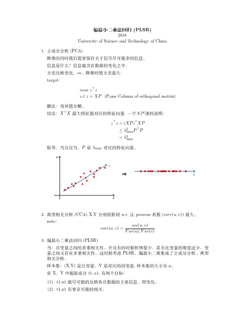
偏最小二乘法回归(PLSR)2018University of Science and Technology of China1.主成分分析(PCA)降维的同时我们需要保存关于信号尽可能多的信息。
信息是什么?信息蕴含在数据的变化之中。
方差反映变化,so ,降维时使方差最大.target:max z ⊤zs.t z =XP (P,one Column of orthogonal matrix)解法:奇异值分解。
结论:X ⊤X 最大特征值对应的特征向量.一个不严谨的说明:z ⊤z =(XP )⊤XP≤λ2max P ⊤P=λ2max取等,当且仅当,P 是λmax 对应的特征向量。
2.典型相关分析(CCA)X,Y 分别投影到u,v.让pearson 系数(corr (u,v ))最大。
note :corr (u,v )=cov (u,v )V ar (u ),V ar (v )3.偏最小二乘法回归(PLSR)当:自变量之间的多重相关性。
并且有的时候样例很少,甚至比变量的维度还少,变量之间又存在多重相关性。
这时候考虑PLSR 。
偏最小二乘集成了主成分分析、典型相关分析。
样本集:(X,Y)是自变量,Y 是对应的因变量,样本集的大小为n 。
在X ,Y 中提取成分t 1,u 1,有两个目标:(1).t1,u1能尽可能的反映各自数据的主要信息,即变化。
(2).t1,u1有要京可能的相关。
结合(1)(2)即是max cov(t1,u1)=corr(t1,u1)∗var(t1)∗var(u1).提取后对数据进行回归,若能满足要求则结束。
若不能,则对残余信息进行第二轮成分的提取。
过程简述:step1:数据的标准化。
(减均值除以方差)step2:maxmize⟨Xp,Y q⟩s.t:∥p∥=1,∥q∥=1拉格朗日求解:L=p⊤X⊤Y q−λ2(∥p∥22−1)−θ2(∥q∥22−1)∂L∂p=X⊤Y q−λp=0(1)∂L∂q=Y⊤Xp−θq=0(2)Then,(p⊤*1)and(q⊤q(2)),we get:λ=θ把1and2联合并带入:maxmize p⊤λp=λs.t:Y⊤XX⊤Y q=λ2qX⊤Y Y⊤Xp=λ2pi.e求最大的奇异值。
干货|揭开差异代谢物筛选的神秘面纱

干货|揭开差异代谢物筛选的神秘面纱开展代谢组学研究,筛选差异代谢物往往是数据分析中最基本的一项分析内容,但分析方法有很多种,例如PLS-DA法、OPLS-DA法、T检验法、倍数变化法……各位老师可能会困惑:到底该选择哪种分析方法?这些方法的筛选指标都有哪些??每项指标的阈值如何设置???这些指标是否需要同时满足????那么接下来,小迈就为各位老师一一解答这些疑惑。
在代谢组学研究中,最常见的差异代谢物筛选方法主要有以下三种:1.倍数变化法(FC值)2.T检验法(P值、FDR值)3.(O)PLS-DA法(VIP值)倍数变化法倍数变化法即根据代谢物的相对定量或绝对定量结果,计算某个代谢物在两组间表达量的差异倍数(Fold Change),简称FC值。
假设A物质在对照组中定量结果为1,在疾病组中定量结果为3,那么此物质的FC值即为3。
由于代谢物定量结果肯定是非负数,那么FC的取值就是(0, +∞)。
为筛选到差异更为显著的代谢物,小迈提供给各位老师的结果中默认选择的是FC值≥2或≤0.5的物质,此标准设置的较为严格,若因此筛到的差异代谢物较少,可根据需求将差异倍数标准调整为1.5倍或者1.2倍,这两种阈值在代谢组研究相关文章中也是较为常见的。
此外,为呈现更好的作图效果,在分析中通常会对FC值取log2对数,若log2FC≥1,则代表此差异代谢物上调,若log2FC≤-1,则代表此差异代谢物下调。
代谢物差异倍数条形图T检验法T检验,又叫student t 检验(S tudent’s t test),是一种常用的假设检验方法,也是差异代谢物筛选中常见的统计策略之一。
假设检验首先必须要有假设,我们假设某代谢物在A组和B组的含量没有差异(H0,零假设),然后基于此假设,通过t test计算出统计量t值和其对应的p值,如果P-value<0.05,那么说明小概率事件出现了,我们应该拒绝零假设,即A组和B组的含量不一样,即有显著差异。
代谢组学导出差异化合物的方法

代谢组学导出差异化合物的方法代谢组学导出差异化合物的方法概述代谢组学作为研究生物体内代谢产物的一种方法,在生物医学和生命科学领域中具有重要的应用价值。
导出差异化合物是代谢组学研究的核心任务之一,本文将介绍几种常用的方法。
质谱法•液质联用技术(LC-MS)是一种常用的代谢组学分析方法,通过将样品中的代谢产物与质谱技术相结合,实现化合物的分析和鉴定。
该方法可以高效地检测和鉴定差异化合物,并获得它们的质量谱图和碎裂图谱。
–高分辨质谱(HRMS)结合质谱数据库的搜索,可以更准确地确定化合物的结构。
–目标分析与非目标分析相结合,可以同时检测已知和未知的代谢产物,提高代谢组学研究的全面性。
核磁共振法•核磁共振(NMR)是一种无损、非破坏性的分析方法,常用于代谢组学中化合物的结构鉴定和定量分析。
–1D和2D NMR技术可以解析复杂样品中的代谢物,提供其结构及关键官能团的信息。
–结合多元统计分析方法,NMR技术可以将大量的代谢谱图数据进行定量和定性分析,帮助识别差异化合物。
色谱法•色谱法是代谢组学分析中另一种常用的方法,包括气相色谱(GC)和液相色谱(LC)。
–GC-MS技术结合色谱技术和质谱技术,可以分离复杂的代谢产物和鉴定目标化合物。
–LC-MS技术可以采用不同的色谱柱和流动相,实现对不同极性化合物的分析,并提高化合物的检测灵敏度。
生物信息学方法•生物信息学方法在代谢组学研究中也发挥着重要的作用。
–代谢通路分析可以通过比对差异化合物与已知代谢通路之间的关系,推断差异化合物可能的生物学功能和代谢途径。
–反向建模方法可以利用差异化合物的浓度数据和代谢通路网络模型,预测与代谢差异有关的代谢酶和途径。
统计学方法•代谢组学数据的处理和差异化合物的筛选离不开统计学方法。
–主成分分析(PCA)和偏最小二乘判别分析(PLS-DA)可以对代谢组学数据进行降维和聚类,发现差异化合物。
–统计显著性分析(如t检验和方差分析)可以通过比较样品组之间的代谢物浓度差异,确定差异化合物。
R语言实现偏最小二乘回归
{
2. 3
X = t1 p1 ' + …t r p r ' + E r Y = t1 q1 ' + …t r q r ' + F r
( 2. 2 )
y2 , …, y q 分别对 x1 , x2 , …, x p 的回归方程 再把 t i = Xw i 带入( 2. 2 ) 即可得到 y1 , y i = β j1 x1 + …β jp x p ( i = 1 , 2, …, q) 根据交叉验证结果选择模型的成分个数 ( 2. 3 )
4
基于葡萄和葡萄酒理化指标的 PLS 实证分析
葡萄酒是由葡萄精细酿造而成, 因此二者的理化指标之间必然存在一定的联系 . 本文采用 中国 2012 年数学建模大赛 A 题中提供的数据, 对红葡萄酒的理化指标与酿酒红葡萄的理化指 标进行最小二乘法建模分析( 以下的葡萄酒与酿酒葡萄均指红葡萄酒与酿酒红葡萄 ) . 4. 1 建模过程
( 2. 1 )
偏最小二乘建模在 R 软件中的实现及实证分析
105
…, p1p ) , q1 ' = ( q11 , …, q1p ) ; E1 与 F1 是回归方程的残差阵, p1 ' 其中, 回归系数向量 p1 ' = ( p11 , 和 q1 ' 可由简单最小二乘法的原则求得 . Step 3 : 用 E1 与 F1 代替 X 与 Y 进行前两个步骤求得第二对成分, 依次循环. 设 X 的秩为 r( r ≤ p) , 则存在 r 个主成分, 使得
只需求出矩阵 M = X'YY'X 的特征值与特征向量, 其最大特征值 λ1 对应的特征向量即为 所求的 w1 , 目标函数值等于 槡 λ1 . Step 2 : 分别做 y1 , y2 , …, y q 和 x1 , x2 , …, x p 对 t1 的回归
偏最小二乘回归方法(PLS)
偏最小二乘回归方法1 偏最小二乘回归方法(PLS)背景介绍在经济管理、教育学、农业、社会科学、工程技术、医学和生物学中,多元线性回归分析是一种普遍应用的统计分析与预测技术。
多元线性回归中,一般采用最小二乘方法(Ordinary Least Squares :OLS)估计回归系数,以使残差平方和达到最小,但当自变量之间存在多重相关性时,最小二乘估计方法往往失效。
而这种变量之间多重相关性问题在多元线性回归分析中危害非常严重,但又普遍存在。
为消除这种影响,常采用主成分分析(principal Components Analysis :PCA)的方法,但采用主成分分析提取的主成分,虽然能较好地概括自变量系统中的信息,却带进了许多无用的噪声,从而对因变量缺乏解释能力。
最小偏二乘回归方法(Partial Least Squares Regression:PLS)就是应这种实际需要而产生和发展的一种有广泛适用性的多元统计分析方法。
它于1983年由S.Wold和C.Albano等人首次提出并成功地应用在化学领域。
近十年来,偏最小二乘回归方法在理论、方法和应用方面都得到了迅速的发展,己经广泛地应用在许多领域,如生物信息学、机器学习和文本分类等领域。
偏最小二乘回归方法主要的研究焦点是多因变量对多自变量的回归建模,它与普通多元回归方法在思路上的主要区别是它在回归建模过程中采用了信息综合与筛选技术。
它不再是直接考虑因变量集合与自变量集合的回归建模,而是在变量系统中提取若干对系统具有最佳解释能力的新综合变量(又称成分),然后对它们进行回归建模。
偏最小二乘回归可以将建模类型的预测分析方法与非模型式的数据内涵分析方法有机地结合起来,可以同时实现回归建模、数据结构简化(主成分分析)以及两组变量间的相关性分析(典型性关分析),即集多元线性回归分析、典型相关分析和主成分分析的基本功能为一体。
下面将简单地叙述偏最小二乘回归的基本原理。
统计师职称考试多元统计分析与应用考试 选择题 60题

1. 在多元统计分析中,主成分分析的主要目的是什么?A. 减少变量数量B. 增加变量数量C. 提高模型复杂度D. 降低模型复杂度2. 下列哪项不是多元回归分析的假设条件?A. 线性关系B. 正态性C. 独立性D. 等方差性3. 在因子分析中,公因子的数量通常如何确定?A. 主观选择B. 根据特征值大于1的原则C. 随机选择D. 根据样本大小4. 聚类分析中,Ward's方法属于哪一类?A. 层次聚类B. 非层次聚类C. 密度聚类D. 网格聚类5. 在判别分析中,Fisher判别法的主要思想是什么?A. 最大化类间差异B. 最小化类内差异C. 最大化类内差异D. 最小化类间差异6. 多元方差分析(MANOVA)与单因素方差分析(ANOVA)的主要区别是什么?A. 处理单个因变量B. 处理多个因变量C. 处理单个自变量D. 处理多个自变量7. 在结构方程模型(SEM)中,路径分析的主要目的是什么?A. 描述变量间的因果关系B. 描述变量间的相关关系C. 描述变量间的线性关系D. 描述变量间的非线性关系8. 在多维尺度分析(MDS)中,常用的距离度量是什么?A. 欧几里得距离B. 曼哈顿距离C. 切比雪夫距离D. 马氏距离9. 在对应分析中,主要用于分析什么类型的数据?A. 连续数据B. 分类数据C. 时间序列数据D. 混合数据10. 在多元统计分析中,偏最小二乘回归(PLS)主要用于解决什么问题?A. 多重共线性B. 异方差性C. 自相关D. 非线性关系11. 在多元统计分析中,典型相关分析(CCA)主要用于分析什么关系?A. 两个变量组之间的关系B. 单个变量组内部的关系C. 多个变量组之间的关系D. 单个变量与多个变量组之间的关系12. 在多元统计分析中,岭回归主要用于解决什么问题?A. 多重共线性B. 异方差性C. 自相关D. 非线性关系13. 在多元统计分析中,LASSO回归主要用于解决什么问题?A. 多重共线性B. 异方差性C. 自相关D. 变量选择14. 在多元统计分析中,支持向量机(SVM)主要用于解决什么问题?A. 分类问题B. 回归问题C. 聚类问题D. 关联分析15. 在多元统计分析中,随机森林主要用于解决什么问题?A. 分类问题B. 回归问题C. 聚类问题D. 关联分析16. 在多元统计分析中,神经网络主要用于解决什么问题?A. 分类问题B. 回归问题C. 聚类问题D. 关联分析17. 在多元统计分析中,决策树主要用于解决什么问题?A. 分类问题B. 回归问题C. 聚类问题D. 关联分析18. 在多元统计分析中,关联规则挖掘主要用于解决什么问题?A. 分类问题B. 回归问题C. 聚类问题D. 关联分析19. 在多元统计分析中,时间序列分析主要用于解决什么问题?A. 分类问题B. 回归问题C. 聚类问题D. 预测问题20. 在多元统计分析中,生存分析主要用于解决什么问题?A. 分类问题B. 回归问题C. 聚类问题D. 时间至事件的分析21. 在多元统计分析中,贝叶斯网络主要用于解决什么问题?A. 分类问题B. 回归问题C. 聚类问题D. 概率推理22. 在多元统计分析中,马尔可夫链蒙特卡罗(MCMC)主要用于解决什么问题?A. 分类问题B. 回归问题C. 聚类问题D. 概率推理23. 在多元统计分析中,高斯过程回归主要用于解决什么问题?A. 分类问题B. 回归问题C. 聚类问题D. 概率推理24. 在多元统计分析中,核密度估计主要用于解决什么问题?A. 分类问题B. 回归问题C. 聚类问题D. 概率密度估计25. 在多元统计分析中,EM算法主要用于解决什么问题?A. 分类问题B. 回归问题C. 聚类问题D. 参数估计26. 在多元统计分析中,K均值聚类主要用于解决什么问题?A. 分类问题B. 回归问题C. 聚类问题D. 关联分析27. 在多元统计分析中,层次聚类主要用于解决什么问题?A. 分类问题B. 回归问题C. 聚类问题D. 关联分析28. 在多元统计分析中,DBSCAN聚类主要用于解决什么问题?A. 分类问题B. 回归问题C. 聚类问题D. 关联分析29. 在多元统计分析中,谱聚类主要用于解决什么问题?A. 分类问题B. 回归问题C. 聚类问题D. 关联分析30. 在多元统计分析中,自组织映射(SOM)主要用于解决什么问题?A. 分类问题B. 回归问题C. 聚类问题D. 数据可视化31. 在多元统计分析中,主成分回归主要用于解决什么问题?A. 多重共线性B. 异方差性C. 自相关D. 非线性关系32. 在多元统计分析中,偏最小二乘判别分析(PLS-DA)主要用于解决什么问题?A. 分类问题B. 回归问题C. 聚类问题D. 关联分析33. 在多元统计分析中,典型相关分析(CCA)主要用于解决什么问题?A. 分类问题B. 回归问题C. 聚类问题D. 关联分析34. 在多元统计分析中,岭判别分析主要用于解决什么问题?A. 分类问题B. 回归问题C. 聚类问题D. 关联分析35. 在多元统计分析中,LASSO判别分析主要用于解决什么问题?A. 分类问题B. 回归问题C. 聚类问题D. 关联分析36. 在多元统计分析中,支持向量机判别分析(SVM-DA)主要用于解决什么问题?A. 分类问题B. 回归问题C. 聚类问题D. 关联分析37. 在多元统计分析中,随机森林判别分析主要用于解决什么问题?A. 分类问题B. 回归问题C. 聚类问题D. 关联分析38. 在多元统计分析中,神经网络判别分析主要用于解决什么问题?A. 分类问题B. 回归问题C. 聚类问题D. 关联分析39. 在多元统计分析中,决策树判别分析主要用于解决什么问题?A. 分类问题B. 回归问题C. 聚类问题D. 关联分析40. 在多元统计分析中,关联规则挖掘判别分析主要用于解决什么问题?A. 分类问题B. 回归问题C. 聚类问题D. 关联分析41. 在多元统计分析中,时间序列判别分析主要用于解决什么问题?A. 分类问题B. 回归问题C. 聚类问题D. 关联分析42. 在多元统计分析中,生存判别分析主要用于解决什么问题?A. 分类问题B. 回归问题C. 聚类问题D. 关联分析43. 在多元统计分析中,贝叶斯网络判别分析主要用于解决什么问题?A. 分类问题B. 回归问题C. 聚类问题D. 关联分析44. 在多元统计分析中,马尔可夫链蒙特卡罗判别分析主要用于解决什么问题?A. 分类问题B. 回归问题C. 聚类问题D. 关联分析45. 在多元统计分析中,高斯过程回归判别分析主要用于解决什么问题?A. 分类问题B. 回归问题C. 聚类问题D. 关联分析46. 在多元统计分析中,核密度估计判别分析主要用于解决什么问题?A. 分类问题B. 回归问题C. 聚类问题D. 关联分析47. 在多元统计分析中,EM算法判别分析主要用于解决什么问题?A. 分类问题B. 回归问题C. 聚类问题D. 关联分析48. 在多元统计分析中,K均值聚类判别分析主要用于解决什么问题?A. 分类问题B. 回归问题C. 聚类问题D. 关联分析49. 在多元统计分析中,层次聚类判别分析主要用于解决什么问题?A. 分类问题B. 回归问题C. 聚类问题D. 关联分析50. 在多元统计分析中,DBSCAN聚类判别分析主要用于解决什么问题?A. 分类问题B. 回归问题C. 聚类问题D. 关联分析51. 在多元统计分析中,谱聚类判别分析主要用于解决什么问题?A. 分类问题B. 回归问题C. 聚类问题D. 关联分析52. 在多元统计分析中,自组织映射判别分析主要用于解决什么问题?A. 分类问题B. 回归问题C. 聚类问题D. 关联分析53. 在多元统计分析中,主成分回归判别分析主要用于解决什么问题?A. 分类问题B. 回归问题C. 聚类问题D. 关联分析54. 在多元统计分析中,偏最小二乘判别分析(PLS-DA)主要用于解决什么问题?A. 分类问题B. 回归问题C. 聚类问题D. 关联分析55. 在多元统计分析中,典型相关分析(CCA)判别分析主要用于解决什么问题?A. 分类问题B. 回归问题C. 聚类问题D. 关联分析56. 在多元统计分析中,岭判别分析主要用于解决什么问题?A. 分类问题B. 回归问题C. 聚类问题D. 关联分析57. 在多元统计分析中,LASSO判别分析主要用于解决什么问题?A. 分类问题B. 回归问题C. 聚类问题D. 关联分析58. 在多元统计分析中,支持向量机判别分析(SVM-DA)主要用于解决什么问题?A. 分类问题B. 回归问题C. 聚类问题D. 关联分析59. 在多元统计分析中,随机森林判别分析主要用于解决什么问题?A. 分类问题B. 回归问题C. 聚类问题D. 关联分析60. 在多元统计分析中,神经网络判别分析主要用于解决什么问题?A. 分类问题B. 回归问题C. 聚类问题D. 关联分析1. A2. C3. B4. A5. A6. B7. A8. A9. B10. A11. A12. A13. D14. A15. A16. A17. A18. D19. D20. D21. D22. D23. B24. D25. D26. C27. C28. C29. C30. D31. A32. A33. A34. A35. A36. A37. A38. A39. A40. A41. A42. A43. A44. A45. A46. A47. A48. A49. A51. A52. A53. A54. A55. A56. A57. A58. A59. A60. A。
偏最小二乘法(PLS)简介

Ah+1=LS的T由公式T=XW计算出,B由公式B=WQ'计算。
相关文献
许禄,《化学计量学方法》,科学出版社,北京,1995。
王惠文,《偏最小二乘回归方法及应用》,国防科技出版社,北京,1996。
Chin, W. W., and Newsted, P. R. (1999). Structural Equation
Akron, Ohio: The University of Akron Press.
Fornell, C. (Ed.) (1982). A Second Generation Of Multivariate
Analysis, Volume 1: Methods. New York: Praeger.
Principal Components Analysis Is To Common Factor Analysis.
Technology Studies. volume 2, issue 2, 315-319.
Falk, R. F. and N. Miller (1992). A Primer For Soft Modeling.
偏最小二乘法(PLS)简介(Partial least squares (PLS))
偏最小二乘法(PLS)简介(Partial least squares (PLS))Introduction to least squares (PLS)| research report | software | training | knowledge sharing | customer directory | BBSIntroduction to least squares (PLS)Number of reading: 14122 release date: 2004-12-30Jane interfaceThe least squares method is a new multivariate statistical analysis method, which was first proposed in 1983 by s.w. old and c.a. lbano. In recent decades, it has developed rapidly in theory, method and application.Partial least squaresFor a long time, the boundaries between model and cognitive methods are well understood. And partial least squares rule them organic combine, under an algorithm, can realize regression modeling (multiple linear regression) at the same time, simplify data structure (principal component analysis (pca) and correlation analysis between the two groups of variables (canonical correlation analysis). This is a leap in the analysis of multivariate statistics.The importance of partial least squares in statistical applications is reflected in the following aspects:Partial least square method is a multidependent variable regression modeling method. The least squares method can solve many problems that can not be solved by ordinary multiple regression.The least square method is called the second generation regression method, and because it can realize the comprehensive application of various data analysis methods.The main purpose of principal component regression is to extract the relevant information hidden in matrix X and then to predict the value of variable Y. This ensures that we only use those independent variables and that the noise will be eliminated to improve the quality of the prediction model. Principal component regression, however, still have some shortcomings, as a useful variable relevance is very small, when we select principal component is easy to miss them, making the final forecast model reliability, if we choose to each component, it is too difficult.Partial least squares regression can solve this problem. It USES the variables X and Y decomposition method, at the same time, extract composition from the variables X and Y (often called a factor), then factors according to the correlation between them from the order. Now, we're going to build a model, and we just have to decide to select a few factors to participate in modelingThe basic conceptPartial least squares regression is an extension of themultiple linear regression model, in its simplest form, using a linear model to describe the independent variables and the relationship between the predictor variable group X: YY = b0 + b1X1 + b2X2 +... + bpXpIn the equation, b0 is the intercept, and the value of bi is the regression coefficient of data point 1 to p.For example, we can think of is a function of his height, gender, weight and from each sample point estimate the regression coefficient, after, we from the measured height and gender can predict someone's weight. For many data analysis methods, the biggest problem is to accurately describe the observed data and make reasonable predictions about new observations.Multiple linear regression model to deal with more complex data analysis problem, expanded the other algorithm, discriminant analysis, principal component regression, correlation analysis, etc., are based on multivariate linear regression model of multivariate statistical methods. These multivariate statistical methods have two important characteristics: the binding of data:The variables X and Y have to be extracted from the X 'X' and Y 'Y matrices, and these factors can't represent the correlation between variables X and Y at the same time.The number of predicted equations should never be greater than the number of variables Y and X.The partial least squares regression is extended from multiple linear regression without the constraint of these data. In the partial least squares regression, the prediction equation is described by the factors extracted from the matrix Y 'xx 'Y. In order to be more representative, the number of prediction equations extracted may be greater than the maximum number of variables X and Y.Partial least-squares regression, in short, may be all in multivariate calibration method for variable constraint minimum method, the flexibility to make it applicable to the traditional multivariate calibration method is not applicable to many occasions, such as some observation data is less than the predicted variables. And, partial least-squares regression can be used as an exploratory analysis tool, before using the traditional linear regression model, to predict the number of the appropriate variable first and remove noise interference.Therefore, partial least-square regression is widely used in many fields for modeling, like chemistry, economics, medicine, psychology and pharmaceutical science and so on, especially it can according to need and arbitrary set a variable that has become more prominent. In stoichiometry, partial least-squares regression has been used as a standard multivariate modeling tool.The calculation processThe basic modelAs a multiple linear regression method, the main purpose of thepartial least-squares regression is to build a linear model: Y = XB + E, which is a m Y variable, n response matrix of sample points, X is a variable p, n sample point prediction matrix, B is the regression coefficient matrix, E correction model to noise, and Y have the same dimension. In general, the variables X and Y are normalized and then used to calculate, minus their average value and divide by the standard deviation.Partial least squares regression and principal component regression, use the factor score as the basis of original prediction variables linear combination, so used to establish the prediction model between factor scores must be linearly independent. For example: if we have a set of response variable Y (matrix) and a large number of prediction variables X (matrix), some of the serious variables linear correlation, we use the extraction factor method factor, extracted from this group of data is used to calculate score factor matrix: T = XW, then find out the appropriate weight matrix W, and establish the linear regression model: Y = TQ + E, the Q is the regression coefficient matrix matrix T, E for error matrix. Once Q is calculated, the previous equation is equivalent to Y = XB + E, where B = WQ, which can be used as a direct regression model.Partial least squares regression and principal component regression method to extract different factor scores in the different, in short, the principal component regression of weight matrix W reflects the predictor variable X, the covariance between the partial least-squares regression of weight matrix W reflects the predictor variable covariance between the response variables X and Y.In modeling, the partial least squares regression produced the weight matrix W of PXC, and the column vectors of matrix W were used to calculate the score matrix T of the NXC of the column vectors of variable X. The constant calculation of these weights has maximized the covariance between the response and its corresponding scoring factors. The normal least-squares regression will generate the matrix Q, the load factor (or weight) of the matrix Y, to set up the regression equation when calculating the regression of Y on T. Once we figure out Q, we can get the equation: Y is equal to XB plus E, where B is equal to WQ, and the final prediction model is set up.Nonlinear iterative partial least squares methodA standard algorithm for calculating partial least squares regression is nonlinear iterative partial least squares (NIPALS), in which there are many variables, some of which are normalized, some of which are not. The algorithm mentioned below is considered to be the most effective of nonlinear iterative partial least squares.H = 1... C, and A0 = X 'Y, M0 = X' X ', C0 = I, and variable c is known.Calculate the main eigenvector of qh, Ah 'ah.Wh is GhAhqh, wh = wh / | | wh | wh |, and wh as the column vector of W.Ph = Mhwh, ch = wh 'Mhwh, ph = ph/ch, and ph is the column vector of P.Qh = Ah 'wh/ch, and qh as the column vector of Q.Ah + 1 = ah-chphqh ', Bh + 1 = Mh - CHPHPH 'Ch + 1 = Ch - WHPH 'The score factor matrix T can be calculated: T = XW, partial least squares regression coefficient B can also be calculated by formula B = WQ.SIMPLS algorithmThere is also an estimation method for partial least-squares regression components, known as SIMPLS algorithm.H = 1... C, and A0 = X 'Y, M0 = X' X ', C0 = I, and variable c is known.Calculate the principal eigenvector of qh and Ah 'ah.Wh = Ahqh, ch = wh 'mhwh, wh = wh/SQRT (ch), and wh as the column vector of W.The ph is the Mhwh, and the ph is the column vector of P.Qh = Ah 'wh and Q h as the column vector of Q.The vh = Chph, vh = vh / | | vh | |Ch + 1 = ch-vhvh ', Mh + 1 = Mh - PHPH 'Ah + 1 = ChAhAs with NIPALS, the T of SIMPLS is computed by formula T = XW, and B is calculated by formula B = WQ '.Related literatureXu lu, methods of stoichiometry, science press, Beijing, 1995.Wang huiwen, the method and application of partial least squares regression. Defense technology press, Beijing, 1996.Chin, w. W., and Newsted, p. r. (1999)Modeling analysis with Small Samples Using Partial LeastC. In Rick Hoyle (Ed.), Statistical Strategies for SmallThe Sample Research, Sage Publications.Chin, w. w. (1998). The partial least squares approach forStructural equation. In George a. Marcoulides (Ed.),Modern Methods for Business Research, Lawrence ErlbaumAssociates.Barclay, D., c. Higgins and r. Thompson (1995). The PartialFurther Squares (PLS) Approach to Causal Modeling: the PersonalComputer Adoption and Use as an illustration. TechnologyStudies, volume 2, issue 2, 285-309.Chin, w. w. (1995). Partial Least Squares Is To LISREL AsPrincipal Components Analysis Is To Common Factor Analysis.Technology Studies. Volume 2, issue 2, 315-319.Falk, r. f. and n. Miller (1992). A Primer For Soft Modeling.By Akron, Ohio: The University of Akron Press.A Second Generation Of MultivariateAnalysis, Volume 1: Methods. New York: Praeger.The last paper: BB model and empirical bayesian methods used in the study of behavioral biasNext: descriptive statistical analysis[close] [print]Contact method |, we are looking for the UK | website navigation Copyright @ 2004 Beijing dyer market research institute Beijing ICP 05033714。
偏最小二乘法原理

偏最小二乘法原理偏最小二乘法(PLS)是一种广泛应用于多元统计分析领域的预测建模方法。
与传统的多元回归方法不同,PLS可以同时考虑多个自变量之间的相关性,以及自变量与因变量之间的关系。
本文将介绍PLS的原理、应用和特点。
一、PLS原理 PLS模型是一种多元线性回归模型,其原理是在自变量和因变量之间选择一组新的变量(称为因子),使得原有变量群中信息方差的损失最小。
这样需要同时考虑自变量之间的相关性和自变量与因变量之间的关系,从而得到有效的预测模型。
具体来说,PLS中的主要思想是将自变量和因变量映射到一个新的空间中,使得在该空间中自变量和因变量之间的协方差最大。
在该过程中,PLS模型会输出一组维度较低的新变量(即因子),这些变量包含了原变量的大部分信息。
最终,基于这些因子建立的多元线性回归模型可以显著提高预测精度。
二、PLS应用 PLS在各个领域都有广泛的应用,尤其是在生化和医学领域中的应用较为广泛。
例如,在药物设计中,PLS可以用来预测分子HIV-1逆转录酶抑制剂活性。
在蛋白质质谱分析中,PLS可以用来识别肿瘤标志物。
在红酒质量控制领域,PLS可以用来评估红酒的年份和产地。
此外,PLS还被应用于图像处理、食品科学、环境科学等领域。
三、PLS特点 1. PLS是一种预测模型,可以应用于多元统计分析领域中的各种问题。
2. PLS可以处理多重共线性的问题,且不需要删除任何自变量。
3. PLS可以同时对多个自变量进行分析,考虑自变量之间的相关性和自变量与因变量之间的关系,有助于提高预测精度。
4. PLS可以利用大量的自变量,甚至在数据较少的情况下也可以获得较高的预测精度。
5. PLS可以防止模型泛化的问题,并且不受离群值或异常值的影响。
四、总结 PLS是一种广泛应用于多元统计分析领域的预测模型,能够同时考虑自变量之间的相关性和自变量与因变量之间的关系,这使得PLS在处理多重共线性问题时具有优势。
此外,PLS可以应用于许多领域,包括生化、医学、图像处理、食品科学、环境科学等。
PCA有哪些变种

PCA有哪些变种
PCA的变种包括但不限于以下几种:
Kernel PCA(核主成分分析):这是一种能够处理非线性数据的PCA 变种。
通过将数据映射到核空间,然后在这个空间中应用PCA,可以得到数据的非线性主成分。
Sparse PCA(稀疏PCA):这是一种用于稀疏数据的主成分分析方法。
稀疏PCA的主要作用在于产生的低维投影中的每个分量是稀疏的(相较PCA得到了稠密分量的子空间)。
PPCA(概率主成分分析):PPCA假设数据在低维度空间上的投影后,数据的类别信息是随机的,而类别的随机性由一个高斯过程来建模。
FA(因子分析):FA是一种用于识别和估计潜在因素或因子的统计技术,这些因素或因子可以解释观察变量之间的相关性。
FA与PCA有一些相似之处,但FA的目标是识别潜在的公共因子,而PCA是为了降维。
PLS-DA(偏最小二乘判别分析):这是一种用于分类任务的PCA变种。
PLS-DA在降维的同时,也考虑到了分类信息,使得降维后的数据更有利于后续的分类任务。
以上是PCA的一些常见变种,它们在处理不同类型的数据和解决不同的问题时各有优势。
在实际应用中,可以根据具体的数据和任务需求选择合适的方法。