NL-means
图像处理中的图像去噪算法综述

图像处理中的图像去噪算法综述随着现代科技的发展,图像处理在各个领域得到了广泛应用。
然而,由于图像采集过程中受到的噪声干扰,导致图像质量下降,降低了后续处理和分析的准确性和可靠性。
因此,图像去噪算法的研究和应用成为图像处理的重要方向之一。
图像去噪算法的目标是从包含噪声的图像中恢复原始图像,以降低噪声对图像质量的影响。
在实际应用中,图像噪声的类型和分布往往是复杂多样的,因此需要选择适合不同场景的去噪算法。
以下将对几种常见的图像去噪算法进行综述。
1. 统计学方法统计学方法通过建立噪声的统计模型来进行图像去噪。
常用的统计学方法包括高斯滤波、中值滤波和均值滤波。
高斯滤波是一种线性滤波器,通过对图像进行平滑处理来减少噪声。
中值滤波则是通过取窗口内像素的中值来代替当前像素值,从而降低噪声的影响。
均值滤波是将像素周围邻域内像素的平均值作为当前像素的新值。
2. 基于小波变换的方法小波变换是一种将信号分解成多个频带的方法,可以对图像进行多尺度分析。
基于小波变换的图像去噪方法通过去除高频小波系数中的噪声信息来恢复原始图像。
常用的小波去噪算法有基于硬阈值法和软阈值法。
硬阈值法通过对小波系数进行阈值处理,将小于阈值的系数设为0,大于阈值的系数保留。
而软阈值法在硬阈值法的基础上引入了一个平滑因子,将小于阈值的系数降低到一个较小的值。
3. 基于局部统计的方法基于局部统计的方法利用图像局部区域的统计特性来去除噪声。
其中,非局部均值算法(NL-means)是一种广泛应用的图像去噪算法。
NL-means 算法通过从图像中寻找与当前像素相似的局部区域,然后根据这些相似区域的信息对当前像素进行去噪。
该算法的优点是对各种类型的噪声都有较好的去除效果,并且能够保持图像的细节信息。
4. 基于深度学习的方法近年来,深度学习在各个领域得到了广泛应用,包括图像去噪领域。
基于深度学习的图像去噪方法通过训练一个适应性的神经网络来学习图像噪声和图像的复杂关系,从而实现去噪效果。
非局部均值图像去噪算法

若需要附件请联系: QQ:2013198460 E_mail:juefeiimage@
式中, I 为受噪声污染的图像; NL 为经过 NL-means 图像去噪后的图像; ni (i 1, 2,3) 表示图像 的第 ni ( ni 为像素点坐标)个像素点, I (ni ) 为其对应灰度值, R(ni ) 和 S (ni ) 分别为以 ni 为中心的相 似窗和搜索窗; (n1 , n2 ) 和 d (n1 , n2 ) 分别表示 R(n1 ) 与 R(n2 ) 相似程度和欧氏距离(两个图像块的欧 式距离为两图像块差的平方和) , h 为衰减参数。 (2)非局部均值算法中参数设置 非局部均值一共有 3 个参数:相似窗 R(ni ) 的大小、搜索窗 S (ni ) 的大小、衰减参数 h 的取值。 这三个参数取值是相互影响,共同作用于 NL-means 的去噪效果:相思窗 R(ni ) 的取值决定使用多大 的窗口进行相似性度量,相似窗过小时大部分相似窗之间的欧氏距离相近,无法区分是否相似,过 大时计算复杂度过高;搜索窗 S (ni ) 的取值决定使用多大的窗口寻找相似窗, 搜索窗过小时可能找不 到足够的相似窗,过大时则计算复杂度过高,理论上,搜索窗为全图时去噪效果最好,但事实并非 这样,搜索窗过大反而会使去噪精度下降(欧氏距离度量相似性的原因) ;衰减参数 h 实际是一个阈 值的作用,当两个相似窗的欧式距离小于 h 时则判定为相似(占得权重 (n1 , n2 ) 较大) ,否则判定为 不相似 (占的权重 (n1 , n2 ) 较小) 。 因此, 增大相似窗 R(ni ) 的大小, 减小 h 的大小, 增大搜索窗 S (ni ) 的大小, 三者对 NL-means 去噪精度的提升可达到同样的效果。 前人大量实验得到三个参数的取值:
声呐信号处理算法

声呐信号处理算法是指对声呐信号进行一系列处理步骤的算法,主要包括信号的采集、预处理、特征提取和分类识别等。
在声呐信号处理中,常用的算法包括非局部均值(NL-means)去噪、BM3D、SAR-BM3D 等方法。
这些方法主要应用于对声呐图像进行去噪处理,以最大程度地保持图像的细节特征。
其中,非局部均值方法的基本思想是:当前像素的估计值由图像中与它具有相似邻域结构的像素加权平均得到。
BM3D 和SAR-BM3D等算法则是在BM3D算法的基础上,结合SAR图像的特点进行改进,用于对SAR图像进行去噪处理。
另外,深度学习技术也被广泛应用于声呐信号处理中。
例如,基于卷积神经网络(CNN)的算法可以用于对声呐信号进行分类、聚类等处理。
这些算法可以通过学习输入数据的统计规律来得出识别结果,有效地对声呐信号进行处理和分析。
除此之外,还有一些其他的声呐信号处理算法,如短时傅里叶变换(STFT)、小波变换(Wavelet Transform)等。
这些算法可以用于对声呐信号进行时频分析、特征提取等处理。
总的来说,声呐信号处理算法是声呐技术中非常重要的组成部分,可以有效地对声呐信号进行处理和分析,为后续的目标识别、分类等任务提供有力的支持。
图像去噪算法:NL-Means和BM3D

图像去噪算法:NL-Means 和BM3D图像去噪是⾮常基础也是⾮常必要的研究,去噪常常在更⾼级的图像处理之前进⾏,是图像处理的基础。
可惜的是,⽬前去噪算法并没有很好的解决⽅案,实际应⽤中,更多的是在效果和运算复杂度之间求得⼀个平衡,再⼀次验证了我⽼师的⼀句话:所有的⼯程问题最后都是最优化问题。
好了,废话不多说,来看看效果⽐较好的去噪算法吧。
噪声模型图像中噪声的来源有许多种,这些噪声来源于图像采集、传输、压缩等各个⽅⾯。
噪声的种类也各不相同,⽐如椒盐噪声,⾼斯噪声等,针对不同的噪声有不同的处理算法。
对于输⼊的带有噪声的图像v(x),其加性噪声可以⽤⼀个⽅程来表⽰:其中是原来没有噪声的图像。
是像素集合,是加项噪声项,代表噪声带来的影响。
是像素的集合,也就是整幅图像。
从这个公式可以看出,噪声是直接叠加在原始图像上的,这个噪声可以是椒盐噪声、⾼斯噪声。
理论上来说,如果能够精确地获得噪声,⽤输⼊图像减去噪声就可以恢复出原始图像。
但现实往往很⾻感,除⾮明确地知道噪声⽣成的⽅式,否则噪声很难单独求出来。
⼯程上,图像中的噪声常常⽤⾼斯噪声来近似表⽰,其中,是噪声的⽅差,越⼤,噪声越⼤。
⼀个有效的去除⾼斯噪声的⽅式是图像求平均,对N 幅相同的图像求平均的结果将使得⾼斯噪声的⽅差降低到原来的N 分之⼀,现在效果⽐较好的去噪算法都是基于这⼀思想来进⾏算法设计。
NL-Means 算法NL-Means 的全称是:Non-Local Means ,直译过来是⾮局部平均,在2005年由Baudes 提出,该算法使⽤⾃然图像中普遍存在的冗余信息来去噪声。
与常⽤的双线性滤波、中值滤波等利⽤图像局部信息来滤波不同的是,它利⽤了整幅图像来进⾏去噪,以图像块为单位在图像中寻找相似区域,再对这些区域求平均,能够⽐较好地去掉图像中存在的⾼斯噪声。
NL-Means 的滤波过程可以⽤下⾯公式来表⽰:在这个公式中,是⼀个权重,表⽰在原始图像中,像素 和像素 的相似度。
基于非局部均值滤波的SAR图像去噪_易子麟
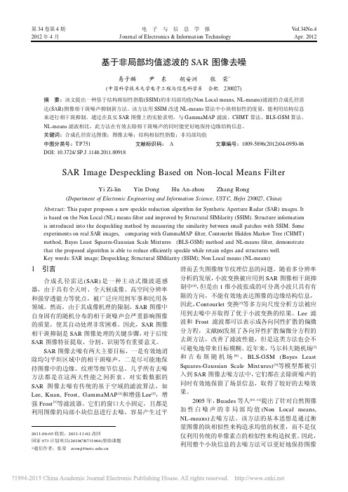
第34卷第4期电子与信息学报Vol.34No.4 2012年4月Journal of Electronics & Information Technology Apr. 2012基于非局部均值滤波的SAR图像去噪易子麟尹东胡安洲张荣*(中国科学技术大学电子工程与信息科学系合肥 230027)摘要:该文提出一种基于结构相似性指数(SSIM)的非局部均值(Non Local means, NL-means)滤波的合成孔径雷达(SAR)图像相干斑噪声抑制新方法。
该方法用SSIM改进NL-means算法中小块相似性的度量,能利用结构信息来进行相干斑抑制。
通过在真实SAR图像上的实验表明,与GammaMAP滤波、CHMT算法、BLS-GSM算法、NL-means滤波相比,此方法在有效去除相干斑噪声的同时能更好地保持边缘结构信息。
关键词:合成孔径雷达图像;图像去噪;结构相似性指数;非局部均值中图分类号:TP751 文献标识码: A 文章编号:1009-5896(2012)04-0950-06 DOI: 10.3724/SP.J.1146.2011.00918SAR Image Despeckling Based on Non-local Means FilterYi Zi-lin Yin Dong Hu An-zhou Zhang Rong(Department of Electronic Engineering and Information Science, USTC, Hefei 230027, China)Abstract: This paper proposes a new speckle reduction algorithm for Synthetic Aperture Radar (SAR) images. It is based on the Non Local (NL) means filter and improved by Structural SIMilarity (SSIM). Structure information is introduced into the despeckling method by measuring the similarity between small patches with SSIM. Some experiments on real SAR images, comparing with GammaMAP filter, Contourlet Hidden Markov Tree (CHMT) method, Bayes Least Squares-Gaussian Scale Mixtures (BLS-GSM) method and NL-means filter, demonstrate that the proposed algorithm is able to reduce efficiently speckle while retain edges and structures well.Key words: SAR image; Despeckling; Structural SIMilarity (SSIM); Non Local means (NL-means)1 引言合成孔径雷达(SAR)是一种主动式微波遥感器,由于具有全天时、全天候成像、高空间分辨率和强穿透能力等优点,被广泛应用到军事和民用各领域。
几种不同权值实现的k-means聚类算法比较
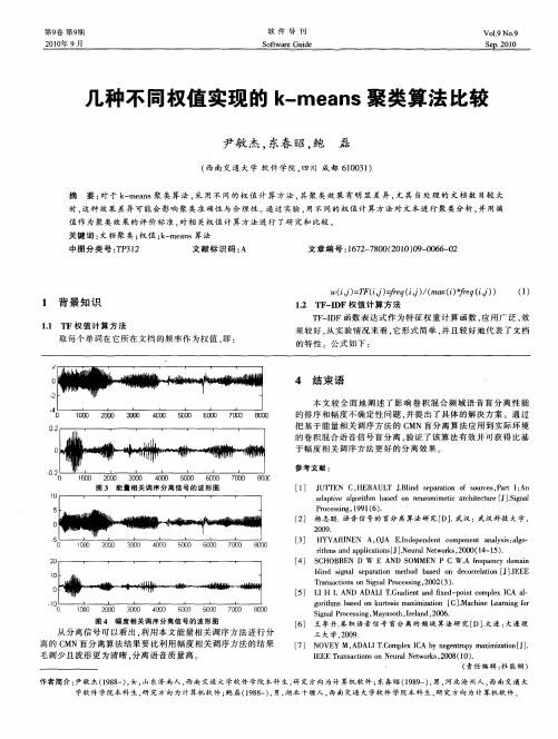
T -D F I F函数 表达 式作 为特征 权重 计算 函数 , 用广 泛 , 应 效 果 较好 , 从实 验情 况来看 , 形式 简单 , 它 并且 较好 地代 表 了文档
的特性 。公式 如下 :
.
I I I L
Ⅱ 0 …l . 4 I l _ _ J . ‘
… … ”
图 4 幅 度 相 关 调 序分 离 信 号 的 波 形 图
[ ] U D AD IT. a i ta df e - on o lxI A a 5 H L AN AL Grde n xd p itcmpe C — n i l gr h ae nk r ssmai zt n [ . c ieL ann r oi msb sdo u oi t t xmi i a o C] Ma hn e rigf o
。 ‘
. . 。。. . ’ . , .
I ’
一
4 结束 语
本文 较 全 面地 阐述 了影 响 卷积混 合 频域 语音 盲 分离 性能 的排 序 和幅度不 确定性 问题 , 提 出了具体 的解决 方案 。通过 并 把 基于能量 相关 调序方 法 的 C MN盲 分离算 法应用 到实 际环境 的卷 积混合 语音信 号盲 分离 , 验证 了该 算法有 效并 可获得 比基 于 幅度 相关 调序 方法更 好 的分离效 果 。
参 考 文 献
11 。 l -
.
口
10 00
2叩 0
30 00
4 0 00
5 0 00
6 0 00
70 00
80 00
[ ] J q ' C, 1 U qEN HER L .l d e aain o ore ,at lAn AU T JBi sprt fsucs P r : n o a a t e agr h ae n n uo mei rhtcue[ ] inl d pi oi m b sd o e rmi t ac i tr J . g a v l t c e S
局部滤波
一个基于当下nonlocal-means图像去噪算法zhaiyao图像去噪是一个至关重要的步骤来提高图像质量和提高性能定量成像分析所需的所有任务。
外地(NL)意味着过滤器去噪图像纹理的一个非常成功的技术。
然而,该算法只是定义了翻译不考虑为每个图像定位和规模补丁。
在本文中,我们介绍了Zernike时刻NL-means过滤器,这是级一组正交复杂图像的时刻。
Zernike时刻在小地方的窗户图像中每个像素计算获得当地的结构信息对于每一个补丁,然后根据这些信息的相似之处而不是像素强度计算。
的旋转不变Zernike时刻,我们可以得到更多的像素或与更高的相似性度量,使补丁相似的补丁平移不变和旋转不变。
该算法是展示了真实图像被高斯白噪声污染)。
比较实验结果表明,改进的NL-means滤波器达到更好的去噪的性能。
关键词:信息检索图像去噪外地意味着过滤器Zernike时刻旋转不变1。
介绍作为图像处理的一个经典问题,图像去噪一直是使用不同的方法来解决。
在同一时间,减少噪声和模糊提出了非线性局部平均方法如非线性扩散过滤器[1]和双边过滤器(2、3)。
最近,Buades et al。
[4]介绍了NLmeans算法,一种新的非线性滤波方法相似邻域滤波。
基于NL-means过滤器周期性的冗余属性图像、纹理图像或自然图像去除噪声。
该方法本质上是一个社区过滤器,吵闹的greyvalues取而代之的是加权平均(平均)grey-values整个喧闹的形象,权重由邻域相似性的图像吗补丁。
换句话说,NL-means过滤器可以查看附近的一个极端的例子与无限的过滤器内核空间和邻居的相似的地方强度是代替逐点地相似grey-values如常用双边过滤。
在古典NL-means算法,让我代表网格图像的恢复强度NL(u)(我)像素,是所有像素的加权平均强度值的离散噪声图像u = {你(我)|我∈}定义作为问(u)(i)=和参数h作为一定程度的过滤。
它控制指数函数的衰减。
水声技术▏黄海宁等:基于形状特征的水声图像小目标识别方法
⽔声技术▏黄海宁等:基于形状特征的⽔声图像⼩⽬标识别⽅法近年来,⽔下成像技术的⽇渐成熟为⾼分辨率⽔声图像的获得提供了可能,⼈⼯静⽌⼩⽬标的定位与识别技术得到了⼴泛研究。
由于⽬标成像受⽔下复杂环境、⽔底地形以及⽔介质特性的影响较⼤,所获得的⽔声图像存在噪声污染、边缘模糊等问题,因此⽬标识别过程存在⼀定阻碍。
尽管如此,在声呐设备获得的⽔声图像中,⽬标的形状特征仍然⽐较明显,形状特征作为描述⽬标的⼀个关键信息,在⽬标识别过程中发挥着重要作⽤,得到了国内外学者的⼴泛重视。
形状特征识别主要是利⽤⽬标或者周边阴影形状的⼏何特性。
Dura等使⽤超椭圆曲线拟合算法,通过控制超椭圆函数的参数来拟合不同⽬标的阴影形状,从阴影部分的超椭圆函数中提取参数特征,以此实现对⽬标的分类,能够得到较⾼的准确率。
Sinai等利⽤C-V轮廓算法对⽬标及阴影区域分别进⾏分割,提取⽬标区域与阴影之间的距离、⾓度等⼏何参数作为特征,对合成孔径声呐(SAS)图像中的⽬标具有良好的识别效果。
然⽽,随着声呐获取图像的⾓度、⽅位发⽣变化,⽬标的阴影形状会存在较⼤差异甚⾄不存在,通过阴影特征进⾏⽬标识别存在⼀定局限性。
对此,Zhai等通过使⽤瑞利混合模型结合马尔科夫随机场直接对⽬标区域进⾏了分割,以此为基础得到⽬标轮廓,能够获取⽬标的形状特征。
王喜龙等利⽤⽔平集⽅法获得声呐图像中⽬标的⼤概轮廓,在此基础上使⽤⽀持向量机对⽬标进⾏识别,最终得到的识别准确率较⾼,应⽤范围较⼴,但是在相似物体的识别⽅⾯还存在⼀定的误差。
此外,深度神经⽹络在⽬标识别中也发挥了重要应⽤,Williams采⽤卷积神经⽹络对⽔下⼩⽬标进⾏识别,根据有⽆⽬标分为两类,分类效果较好。
朱可卿等使⽤深度神经⽹络的⽅法对⾼分辨率声图⼩⽬标进⾏识别分类,能够获得较⾼的准确率。
为了有效地抑制背景噪声,更好地提取⽬标的形状特征,进⼀步提⾼⽬标识别率,本⽂提出⼀种基于形状特征的⽔声图像⼩⽬标识别⽅法。
基于K均值聚类NL-MEANS算法的超声图像去噪
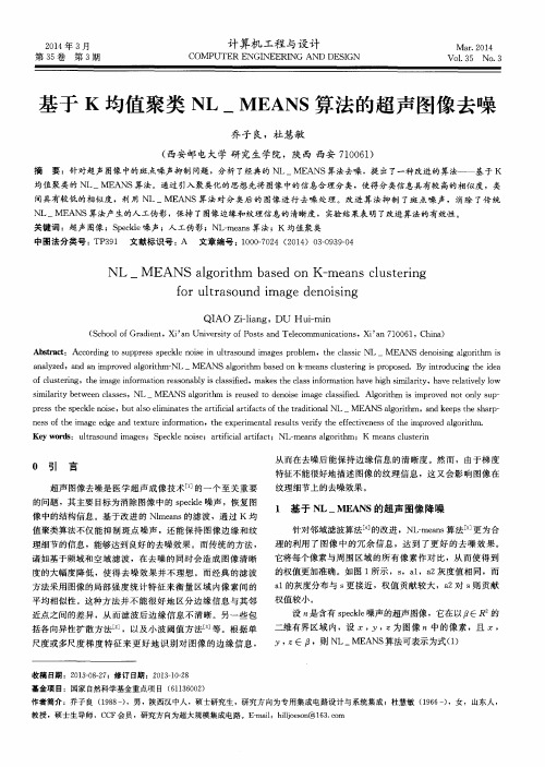
计算机 工程Leabharlann 与设计 COM PUTER ENGI NEERI NG AND DES I GN
Ma r . 2 0 1 4
Vo I . 3 5 No . 3
基于 K均值 聚类 N L—ME A N S算法 的超声图像去噪
乔 子 良 ,杜 慧敏 ( 西安 邮 电 大学 研 究 生学 院 ,陕西 西安 7 1 0 0 6 1 )
a n a l y z e d ,a n d a n i mp r o v e d a l g o r i t h m- NL
— —
M EANS d e n o i s i n g a l g o r i t h m i s
M EA N S a l g o r i t h m b a s e d o n k - me a n s c l u s t e r i n g i s p r o p o s e d .B y i n t r o d u c i n g t h e i d e a
( S e h o o l o f Gr a d i e n t ,Xi ’ a n Un i v e r s i t y o f P o s t s a n d Te l e c o mmu n i c a t i o n s ,Xi ’ a n 7 1 0 0 6 1 ,Ch i n a ) Ab s t r a c t . Ac c o r d i n g t O s u p p r e s s s p e c k l e n o i s e i n u l t r a s o u n d i ma g e s p r o b l e m ,t h e c l a s s i c NL
nl对比词语训练
nl对比词语训练
词向量对比:
- word2vec:基于语言模型的动态表征方法,目标不是语言模型本身,而是词向量,其所作的一系列优化,都是为了更快更好的得到词向量。
- glove:基于全局语料库、并结合上下文语境构建词向量,结合了LSA和word2vec 的优点。
- elmo、GPT、bert:基于语言模型的动态表征方法,可以解决一词多义等问题。
语言模型对比:
- NNLM:所谓分布式假设,用一句话可以表达:相同上下文语境的词有似含义。
- RNNLM:早期词向量的研究通常来源于语言模型,比如NNLM和RNNLM,其主要目的是语言模型,而词向量只是一个副产物。
这些词语在NL领域中具有重要作用,通过对这些词语的学习和理解,可以提高NL处理的能力和水平。
如果你需要更多的NL对比词语训练,请提供更多相关信息,我将尽力为你提供帮助。
基于旋转不变NL—means迭代优化的CT图像POCS重建方法
相片降噪的原理是
相片降噪的原理是
相片降噪的原理是通过算法和技术处理图像中的噪声,从而减少或消除噪声的影响,提高图像的清晰度和质量。
常见的相片降噪原理包括以下几种:
1. 统计滤波:根据图像的统计性质,如均值、方差等,对图像进行滤波处理,去除图像中的噪声。
常用的统计滤波方法有均值滤波、中值滤波等。
2. 非局部均值去噪(NLmeans):通过比较图像的不同区域之间的相似性,对每个像素点进行加权平均,从而降低噪声。
该方法利用了图像中相似纹理区域的统计特性,能够有效去除噪声。
3. 小波去噪:利用小波变换将图像分解为不同频率的子带,对高频子带进行降噪处理,然后再进行逆变换恢复图像。
小波去噪主要用于降低图像的高频噪声。
4. 基于深度学习的降噪:利用深度学习算法,通过训练大量图像样本,学习图像中的噪声和清晰图像之间的映射关系,进而对新的图像进行降噪处理。
这种方法通常需要较大的计算资源和大量的训练样本。
总之,相片降噪的原理是利用图像处理算法和技术,通过对图像的统计特性、纹理特征等进行分析和处理,从而减少图像中的噪声,提高图像的质量和清晰度。
不同的降噪方法适用于不同的噪声类型和降噪要求。
python bm3d用法 -回复

python bm3d用法-回复Python BM3D用法BM3D是一种图像去噪算法,它利用了块匹配(Matching Pursuit)和固有顺序滤波技术(Biorthogonal Orthogonal Multiscale FilterBank)来提高图像的质量。
它可以帮助我们去除图像中的噪声,使图像更加清晰和细节更加明显。
在这篇文章中,我们将详细介绍Python中如何使用BM3D算法,并逐步解释其实现过程。
1. 环境准备在使用BM3D算法之前,我们需要确保已经安装了相应的Python库。
BM3D算法依赖于NumPy、SciPy和OpenCV库。
你可以通过以下命令在终端上安装这些库:pythonpip install numpy scipy opencv-python2. 导入必要的库在程序的开头,我们需要导入BM3D算法所需的库。
这些库将包括NumPy、SciPy和OpenCV。
pythonimport numpy as npfrom scipy import miscimport cv23. 加载图像在对图像进行去噪之前,我们需要首先加载图像。
我们可以使用SciPy 库的`misc.imread()`函数或OpenCV库的`cv2.imread()`函数来加载图像。
下面是使用OpenCV库的示例代码:pythonimage = cv2.imread('image.jpg')4. 调用BM3D算法接下来,我们将使用BM3D算法对图像进行去噪处理。
BM3D算法通常有两个阶段:第一阶段是基于块匹配的3D变换,第二阶段是基于块相似性的去噪。
下面是调用BM3D算法的示例代码:pythonbm3d_denoised = cv2.fastNlMeansDenoisingColored(image,None, 10, 10, 7, 21)在这个示例中,我们使用了`cv2.fastNlMeansDenoisingColored()`函数来调用BM3D算法进行图像去噪。
nlmeans 参数
nlmeans是一种常用的线性模型后向逐步回归方法,可用于拟合线性模型并逐步添加或删除特征。
下面是nlmeans的参数介绍:1. `method`:指定拟合线性模型的方法,常用的有`"lrt"`(逻辑回归)、`"plsr"`(偏最小二乘回归)和`"omp"`(正交最大似然法)等。
2. `family`:指定响应变量的分布类型,常用的有`"gaussian"`(正态分布)、`"poisson"`(泊松分布)和`"binomial"`(二项分布)等。
3. `x_descending`:指定自变量的排序方式,可以按照自变量系数大小进行排序,也可以按照p值大小进行排序。
4. `alpha`:指定阿尔法值,控制逐步回归的步长。
阿尔法值越大,逐步回归的步长越小,即保留的变量越少;阿尔法值越小,逐步回归的步长越大,即保留的变量越多。
5. `method.cond`:指定条件化方法,常用的有`"plsr"`(偏最小二乘回归)和`"omp"`(正交最大似然法)等。
6. `use_std`:指定是否使用标准误,默认为`True`。
7. `x_method`:指定自变量的拟合方法,常用的有`"centered"`(中心化自变量)和`"standardized"`(标准化自变量)等。
8. `y_method`:指定响应变量的拟合方法,常用的有`"centered"`(中心化响应变量)和`"standardized"`(标准化响应变量)等。
9. `max_iter`:指定最大迭代次数,默认为1000次。
10. `n_iter_no_change`:指定连续不改变模型参数的最大迭代次数,默认为10次。
bm4d_preprint
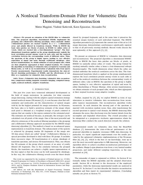
1 A Nonlocal Transform-Domain Filter for V olumetric DataDenoising and ReconstructionMatteo Maggioni,Vladimir Katkovnik,Karen Egiazarian,Alessandro FoiAbstract—We present an extension of the BM3Dfilter to volumetric data.The proposed algorithm,denominated BM4D,implements the grouping and collaborativefiltering paradigm,where mutually similar d-dimensional patches are stacked together in a(d+1)-dimensional array and jointlyfiltered in transform domain.While in BM3D the basic data patches are blocks of pixels,in BM4D we utilize cubes of voxels,which are stacked into a four-dimensional“group”.The four-dimensional transform applied on the group simultaneously exploits the local correlation present among voxels in each cube and the nonlocal correlation between the corresponding voxels of different cubes.Thus, the spectrum of the group is highly sparse,leading to very effective separation of signal and noise through coefficients shrinkage.After inverse transformation,we obtain estimates of each grouped cube,which are then adaptively aggregated at their original locations.We evaluate the algorithm on denoising of volumetric data corrupted by Gaussian and Rician noise,as well as on reconstruction of phantom data from sparse Fourier measurements.Experimental results demonstrate the state-of-the-art denoising performance of BM4D,and the effectiveness of our filter as a regularizer in volumetric data reconstruction.Index Terms—Volumetric data denoising,volumetric data reconstruc-tion,compressed sensing,magnetic resonance imaging,computed tomog-raphy,nonlocal methods,adaptive transformsI.I NTRODUCTIONThe pastfive years have witnessed substantial developments in thefield of image restoration.In particular,for what concerns image denoising,starting with the adaptive spatial estimation strategy termed nonlocal means(NLmeans)[1],it soon became clear that self-similarity and nonlocality are the characteristics of natural images with by far the biggest potential for image restoration.In NLmeans, the basic idea is to build a pointwise estimate of the image where each pixel is obtained as a weighted average of pixels centered at regions that are similar to the region centered at the estimated pixel. The estimates are nonlocal because,in principle,the averages can be calculated over all pixels of the image.One of the most powerful and effective extensions of the nonlocalfiltering paradigm is the grouping and collaborativefiltering approach incarnated by the BM3D image denoising algorithm[2].The method is based on an enhanced sparse representation in transform domain.The enhancement of the sparsity is achieved by grouping similar2D fragments of the image into 3D data arrays which are called“group”.Collaborativefiltering is a special procedure developed to deal with these3D groups.It includes three successive steps:3D transformation of a group,shrinkage of transform spectrum,and inverse3D transformation.Thus,one obtains the3D estimate of the group which consists of an array of jointly filtered2D fragments.Due to the similarity between the grouped blocks,the transform can achieve a highly sparse representation of the true signal so that the noise can be well separated by shrinkage. In this way,the collaborativefiltering reveals even thefinest details This work was supported by the Academy of Finland(project no.213462, Finnish Programme for Centres of Excellence in Research2006-2011,project no.118312,and project no.129118,Postdoctoral Researcher’s Project2009-2011),and by Tampere Graduate School in Information Science and Engi-neering(TISE).All authors are with the Department of Signal Processing,Tampere University of Technology,P.O.Box553,33101Tampere,Finland(e-mail:fistname@tut.fi)shared by grouped fragments and at the same time it preserves the essential unique features of each individual fragment.The BM3D algorithm presented in[2]represents the current state of the art in2-D image denoising,demonstrating a performance significantly superior to that of all previously existing methods.Recent works discuss the near-optimality of this approach[3],[4].We present an extension of BM3D to volumetric data denoising and reconstruction.The proposed algorithm is denominated BM4D. While in BM3D the basic data patches are blocks of pixels,in BM4D we naturally utilize cubes of voxels.The group formed by stacking mutually similar cubes is hence a four-dimensional orthope (hyperrectangle).The fourth dimension along which the cubes are stacked embodies the nonlocal correlation across the data.The four-dimensional transform which is applied on the group simultaneously exploits the local correlation present among voxels in each cube as well as the nonlocal correlation between the corresponding voxels of different cubes.Like in BM3D,the spectrum of the group is highly sparse,leading to very effective separation of signal and noise by either thresholding or Wienerfiltering.After inverse transformation, we obtain estimates of each grouped cube,which are then aggregated at their original locations using adaptive weights.Further,inspired by[5],[6],we exploit BM4D as form of reg-ularization in iterative volumetric data reconstruction from incom-plete(sparse)measurements.Our reconstruction algorithm works recursively.In each iteration the missing part of the spectrum is injected with excitation random noise;then,after transforming the excited spectrum to spatial voxel domain,the BM4D denoisingfilter attenuates the noise,thus disclosing even the faintest details from the incomplete and degraded observations.The overall procedure can be interpreted as a progressive stochastic approximation where the denoisingfilter conducts the search direction towards the solution. Experimental results on volumetric data from the BrainWeb database[7]demonstrate the state-of-the-art performance of the proposed algorithm in magnetic resonance(MR)data denoising.In particular,we report significant improvement over the results pro-vided by the optimized volumetric implementations of the NLmeans filter[8],[9],[1],which to the best of our knowledge,were up to now the most successful approaches to MR denoising.Moreover,our algorithm allows to achieve excellent reconstruction performance of the synthetic Shepp-Logan phantom even from a very limited number projections,and under different sampling trajectories,as the ones presented in[10].The remainder of paper is organized as follows.In Section II we formally define the BM4D algorithm and the adopted observation model.Section III is devoted to the discussion of the employed parameters,while the denoising experimental results are analyzed in Section IV.In Section V wefirst describe the iterative reconstruction algorithm and then report its experimental validation.Concluding remarks are given in Section VI.2II.BM4D A LGORITHMA.Observation ModelWe consider the noisy volumetric observation z:X→R asz(x)=y(x)+η(x),x∈X,(1) where y is the original,unknown,volumetric signal,η(·)∼N(0,σ2) is i.i.d.additive white Gaussian noise having varianceσ2assumed known a priori,and x=(x1,x2,x3)is a3-D spatial position belonging to the domain X⊂Z3.B.ImplementationThe objective of the proposed volumetric data denoising algorithm is to provide an estimateˆy of the original y from the noisy observation z.Similar to the BM3D algorithm,also BM4D is implemented in two cascading stages,namely hard-thresholding and Wienerfiltering stage,each comprising three steps:grouping,collaborativefiltering, and aggregation.Let C z xR denote a cube of size L×L×L,with L∈N,extractedfrom z at the3-D spatial location x R∈X,which identifies its top-left corner.In the hard-thresholding stage,the four-dimensional groups are formed by stacking together,along an additional fourthdimension,(three-dimensional)cubes similar to C z xR extracted fromthe noisy volumetric data z.Specifically,the similarity between two cubes is measured as the squared 2-norm of the intensities difference of their voxels normalized with respect to the size of the cube support asd `C z xi,C z xj´=˛˛˛˛C z xi−C z xj˛˛˛˛22L3.(2)In BM4D,two cubes are considered similar if their distance(2)is smaller or equal than a predefined thresholdτht match.Thus,the set containing the indices of the cubes extracted from z that are similar to C z xRis defined asS z xR =nx i∈X:d(C z xR,C z xi)≤τht matcho.(3)In the grouping,we use the set S z xR to build the four-dimensionalgroup associated to the reference cube C z xRasG z S zx R =˘C z xi:x i∈S z xR¯.(4)Observe that,since d(C z xR ,C z xR)=0,each set G z xRnecessarilycontains at least one cube,that is C z xRitself.During collaborativefiltering,atfirst each group G z S zx Ris trans-formed by a decorrelating separable four-dimensional transform T ht4D, then the spectrum coefficients are shrunk through a hard-thresholding operatorΥht with threshold valueσλ4D,and thefiltered group ˆG yx Ris eventually produced by inverting the original transform T ht4D. FormallyˆG yS z xR =T ht−14D“Υht“T ht4D“G z S zx R”””,(5)thus producingˆG yS z xR =˘ˆC y xi:x i∈S z xR¯,(6)where eachˆC y xi is an estimate of the original C y xiextracted from theunknown volumetric data y.Since the cubes in the different groupsˆG yS z xR (as well as the cubeswithin the same group)are likely to overlap,we may have multiple estimates for the same voxel.Therefore thefinal volumetric estimate ˆy ht is obtained through a convex combination with adaptive weights (“aggregation”)ˆy ht=Px R∈X“Px i∈S z xRw ht xRˆC yx i”Px R∈X“Px i∈S z xRw ht xRχxi”,(7)whereˆC y xiis assumed to be zero-padded outside its domain,and χxi:X→{0,1}is the characteristic function of the support of the cubeˆC y xi.The aggregation weights w ht xRare defined to be inversely proportional to the total sample variance of the estimate of the corresponding groups,which is approximated by the number N ht xRof non-zero coefficients in the spectrum ofˆG yS z xR[2].In the Wienerfiltering stage,the grouping is performed within the hard-thresholding estimateˆy ht,thus for each reference cube Cˆy ht xRwith x R∈X we computeSˆy ht xR=x i∈X:˛˛˛˛Cˆy ht xR−Cˆy ht xi˛˛˛˛22L3<τwiematchff.(8) In this manner,since the noise in the basic estimate can be assumed considerably reduced,we improve the accuracy of cube-matching, consequently benefiting the quality offiltering because the spectra of the groups are better sparsified by the increased correlation of the underlying grouped data.The set of coordinates Sˆy ht xRis used to form two groups:one from the observation z,and the other from the basic estimateˆy ht,termed G zSˆyhtx Rand Gˆy htSˆyhtx R,respectively.The empirical Wiener shrinkage coefficients are defined from the energy of the transformed spectrum of the basic estimate group asWSˆyhtx R=˛˛˛T wie4D“Gˆy htSˆyhtx R”˛˛˛2˛˛˛T wie4D“Gˆy htSˆyhtx R”˛˛˛2+σ2.(9)Collaborativefiltering is then realized through element-by-element multiplication between the group spectrum and the shrinkage coef-ficients(9).The group of cube estimates is thereafter produced byinverting the four-dimensional transform T wie4DasˆG ySˆyhtx R=T wie−14D“WSˆyhtx R·T ht4D“G zSˆyhtx R””.(10)Thefinal estimateˆy wie is produced through a convex combination, as in(7),where the set S z xRis replaced with Sˆy ht xR,and the aggregation weights for a specific group G zSˆyhtx Rarew wie xR=˛˛˛˛˛˛WSˆyhtx R˛˛˛˛˛˛−22,(11) being the total variance estimate of the Wienerfiltered group[2].III.A LGORITHM P ARAMETERSWe set the size L of the cube,such that the size of support of the d-dimensional patch of BM4D(the cube)would have been equal to the support of the d-dimensional element of BM3D(the block). BM3D is presented under two sets of parameter:the normal and modified profile[2],in which the blocks have size8×8and11×11, respectively.Thus,we set L=4and L=5in the correspondent two parameters sets of BM4D,so that the size of the support of the patches is roughly the same.As a matter of fact,we are able to successfully utilize most of the settings originally optimized for BM3D.The separable four-dimensional transforms are similar to those in [2],particularly in the hard-thresholding stage T ht4D is a composition3 TABLE IP ARAMETER SETTINGS FOR THE PROPOSED BM4D ALGORITHM.Param.StageHard thresholding Wienerfiltering Normal Modif.Normal Modif.Cube size L445Group size M163232Step N step3Search-cube size N S11Similarity thr.τmatch3000250004003500Shrinkage thr.λ4D 2.7 2.8Unusedof a3-D biorthogonal spline wavelet in the spatial dimensions with a1-D Haar wavelet in the grouping dimension.The Wienerfiltering stage employs in the spatial dimensions a3-D DCT.The Haar transform in the fourth dimension restricts the cardinality of the groups to be a power of two,but since such cardinality is not known a priori,we constrain the number of grouped cubes to be the largest power of2smaller than or equal to the minimum value between the original cardinality of the groups and a predefined value stly,in order to reduce the computational complexity of the algorithm,the grouping is performed within a three-dimensional window of size N S×N S×N S centered at the coordinate of the current reference cube,and all such reference cubes are separated by a step N step∈N in every spatial dimension.The modified parameters are set following the comments suggested in[11],which should benefit volumetric denoising with aggressive noise levels.The modifications aim to create larger groups in the both stages,by increasing the thresholdsτand the cardinality M,and to use slightly bigger cubes,to enhance the reliability of matching in case of large noise variance.Table I summarizes all the parameters employed in BM4D for both profiles,together with their relative values.IV.D ENOISING E XPERIMENTSThe effectiveness of the proposed BM4D algorithm is verified by means of its denoising performance on magnetic resonance(MR) images,as they are one of the most prominent examples of volumetric data from real-world applications.As quality measure,we compute the PSNR of the denoised data asPSNR=10log102552|˜X|Px∈˜X(ˆy wie(x)−y(x))2!,(12)where˜X={x∈X:y(x)>10}(in oder not to compute the PSNR on the background as in[12]),and|˜X|is the cardinality of˜X. A.DenoisingThe experiments are made under both Gaussian and Rician dis-tributed noise,using the T1brain phantom of size181×217×181 voxels from the BrainWeb database[7]as volumetric test data. As a comparison,we validate the denoising performances of the proposed BM4D algorithm against the optimized blockwise nonlocal means with wavelet mixing OB-NLM3D-WM presented in[12],as it represents,to the best of our knowledge,the state of the art in MR image denoising.According to(1),we synthetically generate the noisy observations z by adding white Gaussian noise having different values of standard deviationσ,ranging from1%to23%of the maximum value of the signal y.In practice,since we assume to deal with signals normalized to the range[0,255],σvaries from2.55to58.65.1357911131517192123 283032343638404244σ(%)PSNR(dB)1357911131517192123 283032343638404244σ(%)PSNR(dB)Fig.1.PSNR performances of the BM4D denoisingfilter applied to the BrainWeb phantom[7]corrupted by i.i.d.Gaussian noise(top)and Rician noise(bottom)with varying level ofσ.For each noise distribution there are reported the results BM4D tuned with the normal(◦)and the modified( ) parameters,as described in Section III(see Table I).The results present a consistent behavior with Figure9in[2],where different profiles are compared in2-D image denoising.Leveraging a recently proposed method of variance-stabilization (VST)[13]for the Rice distribution,the proposed BM4D algorithm can be applied also to Rician-distributed data.As in[13],the observation model of a Rician observation z isz(x)∼R(y(x),σ),x∈X,(13) where y is the original signal,and z represents the raw magnitude MR data,and R(ν,σ)denotes the Rician distribution withν≥0 andσ>0.The OB-NLM3D-WM algorithm exists in separate implementations developed for Gaussian and for Rician distributed noise,thus we decorate their names with a subscript“N”(Gaussian) and“R”(Rician)to denote the noise distribution addressed by the specific algorithm implementation.Wefirst present the denoising results in terms of PSNR of the BM4Dfilter under the normal and modified profile,whose parameters are reported in Table I.Figure1shows the progression of the PSNR as the standard-deviationσof the noise(for both Gaussian-and Rician-distributed data)increases.As one can see,the modified set of parameters dominates the normal profile under any level ofσin both distribution,and it provides a substantial gain especially when σ>15%.These results are explained by the nature of MR images, as modeled by the BrainWeb phantom,predominantly characterized by low-frequency content,abundance of similar patches,and a vast smooth background.The modified profile leverages such attributes,4TABLE IIPSNR DENOISING PERFORMANCES ON THE VOLUMETRIC TEST DATA FROM THE B RAIN W EB DATABASE [7]OF THE PROPOSED BM4D (TUNED WITH THE MODIFIED PROFILE )AND THE OB-NLM3D-WM [12]FILTER .T WO KINDS OF OBSERVATIONS ARE TESTED ,ONE CORRUPTED BY I .I .D .G AUSSIAN AND THE OTHER BY SPATIALLY HOMOGENOUS R ICIAN NOISE ACCORDING TO THE OBSERVATION MODELS (1)AND (13).B OTH CASES ARE TESTED UNDER TWELVE STANDARD -DEVIATIONS σ,EXPRESSED AS PERCENTAGE RELATIVE TO THE MAXIMUM INTENSITY VALUE OF THE ORIGINAL VOLUMETRIC DATA .VST REFERS TO THE VARIANCE -STABILIZATION FRAMEWORK DEVELOPED FOR R ICIAN -DISTRIBUTED DATA [13].T HE SUBSCRIPTS N(G AUSSIAN )AND R (R ICIAN )DENOTE THE ADDRESSED NOISE DISTRIBUTION .NoiseFilterσ1%3%5%7%9%11%13%15%15%17%21%23%Gaussian BM4D44.0938.4035.9534.3833.2132.2631.5030.8230.2429.7029.2028.77OB-NLM3D-WM N42.4437.7335.0433.1831.8030.6929.7728.9828.2827.6627.0926.57RicianVST +BM4D 44.0838.3335.8334.1732.8831.8130.8730.0529.2728.5627.9127.26OB-NLM3D-WM R 42.3737.5434.7232.7131.1429.8228.6727.6526.7225.8625.0724.33VST +OB-NLM3D-WMN42.4637.6834.8232.7931.2630.0429.0228.1427.3526.6325.9725.36Original Noisy OB-NLM3D-WM BM4DFig.2.From left to right,original cross-section of the test brain phantom from the BrainWeb database [7],noisy cross-section corrupted by i.i.d.Gaussian noise with standard deviation σ=38.25(15%),and corresponding denoised results of the OB-NLM3D-WM [12],and the proposed BM4D filter.For each phantom,both the 3-D and 2-D transversal cross-section are presented in the top and bottom row,respectively.because,on one hand,it is generally aimed at building bigger groups with the maximum possible cardinality,and,on the other,it apply a slightly more aggressive smoothing by increasing the threshold parameter λ4D .That being so,we choose to apply the modified parameters to BM4D for all cases of our experimental evaluation.Table II reports the PSNR outputs of the abovementioned filters.The proposed BM4D algorithm achieves better performances than the OB-NLM3D-WM filter both under Gaussian and Rician distributed noise,with a consistent improvement of at least 1dB.Additionally,observe that for levels of noise σ≤15%the performance losses of the experiments under Rician noise with respect to the corresponding Gaussian results are similar for both algorithms,although being slightly smaller in BM4D.However,OB-NLM3D-WM R is subjected to significantly larger decays of performance when σenlarges.Figure 2shows a cross-section of the test brain phantom,denoised by the two algorithms;the noisy observation has been corrupted by white Gaussian noise having σ=38.25(15%).BM4D achieves an excellent visual quality in the restored phantom,as can be seen from the smoothness in flat areas,the details preservation along edges,and the accurate intensity preservation.V.I TERATIVE R ECONSTRUCTION FROM S PARSE M EASUREMENTS A.Problem SettingIn volumetric reconstruction,an unknown signal of interest is observed (sensed)through a limited number linear functionals.In compressed-sensing problems,these observations can be considered as a sparse portion of the spectrum of the signal in transform domain.Therefore,the direct application of an inverse transform cannot in general reconstruct the signal,as compressed sensing considers cases where the available spectrum is much smaller than what is required according to the Nyquist-Shannon sampling theory.However,it is generally assumed that the signal can be represented sparsely in a suitable transform domain,and in [5],[6],it is shown that under such assumptions,stable reconstruction of the unknown signal is possible and that in some cases the reconstruction can be exact.Typical techniques rely on convex optimization with a penalty ex-pressed by the 0or 1norm which is exploited to enable the assumed sparsity [14],[15].It results in parametric modeling of the solution and in problems that are then solved by mathematical programming algorithms.Our approach replaces the parametric modeling with a nonparametric one implemented by the use of a spatially adaptive denoising filter [6].17%19%________5We denote by y the unknown original volumetric signal,and by θ=T (y )its corresponding representation in transform domain.For our purposes,θcan be either composed by the 2-D Fourier transforms of every cross-section of the phantom y ,or it can be the 3-D Fourier spectrum of y ,thus simulating real-world magnetic resonance or computed tomography acquisition [16],[10].If we had the complete spectrum θ,we could easily invert the transformation and obtain exactly the original signal as y =T −1(θ).However,only a small portion of the spectrum θis available,thus the reconstruction of y is an ill-posed problem.Let S be a 3-D sampling operator that is applied to the acquired volumetric signal θ.We define S as the characteristic (indicator)function of the available portion Ωof the spectrum,thus S =χΩ→{0,1}.By means of the sampling operator S ,we can split the spectrum in two complementary parts asθ=S ·θ|{z}θ1+(1−S )·θ|{z }θ2,(14)where θ1=S ·θand θ2=(1−S )·θare the observed (known)andunobserved (unknown)portion of the spectrum θ,respectively.Our goal is to reconstruct the θ,and consequently y ,from the available portion θ1.B.Volumetric Reconstruction AlgorithmThe reconstruction,is carried out by a recursive system as in [5],[6].Given an estimate ˆθ(k )2of θ2,we define the estimate ˆθ(k )of the complete spectrum θas ˆθ(k )=θ1+ˆθ(k )2,where the superscript k denotes the relative iteration.Initially,we set the estimate of the unobserved θ2to zero,i.e.ˆθ(0)2=0,obtaining the initial back-projection ˆy (0)=T −1`ˆθ(0)´.Each iteration (k ≥1)comprises of two cascading steps:1)Spatial domain volumetric filtering .The reconstructed volumet-ric estimate T −1(ˆθ(k −1))of the previous iteration (k −1)is filtered using an adaptive spatial volumetric filter Φasˆy (k )=Φ“T −1`ˆθ(k −1)´”(15)2)Noise addition (excitation).The estimated unobserved part ˆθ(k )2of the spectrum is excited by the injection of (pseudo)random noise ηk ,so that the additive noise (1−S )·ηk acts as a random generator of the missing components of θ:ˆθ(k )=θ1+ˆθ(k )2·ηk.(16)In the subsequent iteration,such components will be attenuated or enhanced by the action of the filter BM4D,depending to the extent of the agreement with the spatial features of the observed (known)spectrum θ1.The algorithm stops either when the estimate ˆθreaches numerical convergence,or after a specified number of iterations.Note that in the final iteration k final we do not excite the algorithm,thus ηk final =ments and remarks about the convergence of the iterative system and the excitation noise can be found in [5],[6].C.Volumetric Reconstruction ExperimentsIn our experiments,we show the reconstruction results of the iter-ative system described in Section V-B,using BM4D 1in place of the general volumetric filter Φ.The parameters of the filter are the same reported in Section III,however only the first (hard thresholding)stage is employed during the reconstruction.The excitation noise ηk is chosen for simplicity to be i.i.d Gaussian noise with exponentially1Codepublicly available at http://www.cs.tut.fi/∼foi/GCF-BM3D/c =5%c =10%c =20%Fig.3.From top to bottom,the radial,spiral,logarithmic-spiral,limited-angle,and spherical subsampling trajectories of the 3-D sampling operator S ,depending on different coverage level c .decreasing variance Var [ηk ]=α−k −β,with α>0,and β>0,so that the excitation lessens as the iterations increase to prevent excessive smoothing of the small details in the volume.The metric to measure the performance of the reconstruction is the PSNR,as defined in (12).Two sets of experiments are presented,differing in the the number of iterations and in the parameters of the excitation noise.In the first set the algorithm is stopped after 1000iteration and the excitation noise is driven by α=1.02and β=200;in the second one we limit the number of iterations to 100,and the excitation noise decreases faster with α=1.15and β=25.The validation of our experimental results is carried out using a 3-D Shepp-Logan phantom [19]of size 128×128×128voxels,as it is a widely used test data in medical tomography [17],[18].The 3-D sampling operator S can be either composed by a stack of identical 2-D trajectories possibly having different phase,or it can consist of 3-D sampling trajectories (e.g.,as in the bottom row of Figure 3).In the former case,illustrated in Figure 4,the measurements are taken as a stack of 2-D cross-sections transformed in Fourier domain,each of which undergo the sparse sampling induced by the corresponding 2-D trajectory of S .In the latter case,the observation is sampled directly in 3-D Fourier transform domain [10].We present the reconstruction results obtained by five different+(1¡S )¢´k:______6Fig.4.From left to right.Four transversal cross-sections of the original Shepp-Logan phantom,3-D sampling operator S as a stack of four2-D spiral trajectories,and corresponding observed phantom obtained from the sampling induced by S to the phantom.yˆy(0)ˆy(kfinal)Fig.5.From top to bottom,radial,spiral,logarithmic-spiral,limited angle,and spherical reconstruction of the3-D modified Shepp-Logan phantom with subsampling having coverage level c=5%.Both3-D and2-D cross-sections of the original data y,the initial back-projection estimateˆy(0)and thefinal estimateˆy(kfinal)after1000iterations are illustrated.7TABLE IIIPSNR RECONSTRUCTION PERFORMANCES OF THE ITERATIVE SYSTEM DESCRIBED IN S ECTION V-B APPLIED TO THE MODIFIED S HEPP -L OGAN PHANTOM OF SIZE 128×128×128VOXELS .T HE TESTS ARE MADE USING THE SUBSAMPLING TRAJECTORIES ILLUSTRATED IN F IGURE 3,UNDER THREE DIFFERENT COVERAGE LEVELS ,AFTER 1000AND 100ITERATION .Trajectory Iteration Coverage 5%10%20%Radial 100081.63117.02125.0210027.1144.2490.39Spiral 100093.49120.66124.3110021.0328.8350.64Log.Spiral 100095.20123.57126.5110035.6455.5074.03Lim.Angle 100043.7446.0451.5210023.9425.5526.35Spherical1000115.99118.28121.8510036.1150.9792.2310020030040050060070080090010002030405060708090100110IterationP S N R (d B )100200300400500600700800900100024681012Iterationσ(%)Fig.6.The uppermost plot shows the progression of the PSNR of the BM4D reconstruction filter applied to the modified Shepp-Logan phantom subsampled with coverage level c =5%with radial (◦),spiral (+),logarithmic-spiral ( ),limited-angle ( ),and spherical (×)with respect to the number of iterations.The lowermost plot illustrates the standard-deviation σof the excitation noise used in each iteration,expressed as percentage relative to the maximum intensity value of the original volumetric data.trajectories and three different coverage levels c ,i.e.the ratio between the sampled voxels and the total number of voxels in the phantom.The trajectories used in our experiments are radial,spiral,logarithmic-spiral,limited-angle and spherical,as they are widely used in modeling medical imaging acquisition [10].Such trajectories are illustrated with three coverage levels c in Figure 3.The corresponding reconstruction results are presented in Table III and Figure 5,respectively.As one can see,the performances of the BM4D filter in the iterative system described in Section V-B are substantiated by both the PSNR outcomes and the visual appearance of the reconstructed phantom.Figure 6gives a deeper look on the progression of both the excitation noise and the PSNR with respect to the number of iterations.We observe that the reconstruction performance relative to the limited-angle subsampling ceases to increase at about iteration 450,i.e.when the standard-deviation of the excitation noise drops below unity;the same phenomenon,in smaller magnitude,influences the reconstruction with radial subsampling.This is due to the aggressive and unfavorable subsampling of the two trajectories which would require the excitation noise to decrease more gently as the iterations increase,avoiding situations in which the phantom estimate is trapped in a local optimum during the reconstruction.In all the remaining cases the PSNR grows almost linearly with the number of iterations.We remark that the coverage level c is not a fair measure of the difficulty of reconstruction,because different trajectories having the same c extract different coefficients from the Fourier measurements.In particular,a trajectory that samples densely around the DC term would be advantaged during the reconstruction as it can rely on more meaningful information.This phenomena is clearly reported in Table III,where the logarithmic-spiral and the spherical trajectories achieve after 100iterations the higher performances,with gains up to 15dB.VI.D ISCUSSION AND C ONCLUSIONSA.Video vs.Volumetric Data FilteringV olumetric data shares the same dimensionality with standard video,as they both have a 3-D domain.While the first two dimensions identify in both cases the width and the height of the data,i.e.a 2-D spatial domain,the connotation of the third dimension fundamentally differs from each other,as it embodies peculiar meanings in the two different types of data.It represents an additional spatial dimension,the depth,in case of volumetric data,and it represents time,that is the temporal-index of the frame sequence,in case of videos.Because of the same dimensionality,it might seem reasonable to treat volumetric data as if it was a common frame sequence,and thus process it using standard video filtering algorithms.However,we remark the importance of differentiating such types of data,by devising proper filtering methods able to benefit from the specific and peculiar data correlation present in 3-D volumes opposed to the one that characterize videos.The temporal dimension is a key factor that has to be taken into account in video filtering applications,in fact,effective algorithms can be devised by leveraging the motion information present in videos [20].V olumetric data,on the other hand,is intrinsically different from video data,as the temporal dimension is replaced by an additional spatial dimension,therefore the correlation type to be exploited must relate to the local similarity in the 3-D spatial domain.To highlight these differences,we carry out an experiment where we apply the proposed BM4D and the state-of-the-art video filter V-BM4D [20]to the BrainWeb phantom and to the standard test sequence Flower corrupted by i.i.d.Gaussian noise with standard deviation σ={9%,13%}.In Table IV we report the PSNR results of our tests and,as expected,we note that each algorithm performs。
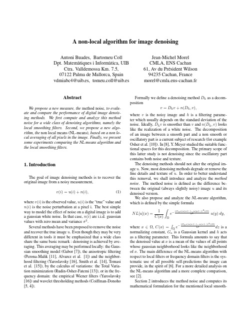
A non-local algorithm for image denoising
A non-local algorithm for image denoisingAntoni Buades,Bartomeu Coll Dpt.Matem`a tiques i Inform`a tica,UIB Ctra.Valldemossa Km.7.5,07122Palma de Mallorca,Spain vdmiabc4@uib.es,tomeu.coll@uib.esJean-Michel MorelCMLA,ENS Cachan 61,Av du Pr´e sident Wilson 94235Cachan,France morel@cmla.ens-cachan.frAbstractWe propose a new measure,the method noise,to evalu-ate and compare the performance of digital image denois-ing methods.Wefirst compute and analyze this method noise for a wide class of denoising algorithms,namely the local smoothingfilters.Second,we propose a new algo-rithm,the non local means(NL-means),based on a non lo-cal averaging of all pixels in the image.Finally,we present some experiments comparing the NL-means algorithm and the local smoothingfilters.1.IntroductionThe goal of image denoising methods is to recover the original image from a noisy measurement,v(i)=u(i)+n(i),(1) where v(i)is the observed value,u(i)is the“true”value and n(i)is the noise perturbation at a pixel i.The best simple way to model the effect of noise on a digital image is to add a gaussian white noise.In that case,n(i)are i.i.d.gaussian values with zero mean and varianceσ2.Several methods have been proposed to remove the noise and recover the true image u.Even though they may be very different in tools it must be emphasized that a wide class share the same basic remark:denoising is achieved by ave-raging.This averaging may be performed locally:the Gaus-sian smoothing model(Gabor[7]),the anisotropicfiltering (Perona-Malik[11],Alvarez et al.[1])and the neighbor-hoodfiltering(Yaroslavsky[16],Smith et al.[14],Tomasi et al.[15]),by the calculus of variations:the Total Varia-tion minimization(Rudin-Osher-Fatemi[13]),or in the fre-quency domain:the empirical Wienerfilters(Yaroslavsky [16])and wavelet thresholding methods(Coiffman-Donoho [5,4]).Formally we define a denoising method D h as a decom-positionv=D h v+n(D h,v),where v is the noisy image and h is afiltering parame-ter which usually depends on the standard deviation of the noise.Ideally,D h v is smoother than v and n(D h,v)looks like the realization of a white noise.The decomposition of an image between a smooth part and a non smooth or oscillatory part is a current subject of research(for example Osher et al.[10]).In[8],Y.Meyer studied the suitable func-tional spaces for this decomposition.The primary scope of this latter study is not denoising since the oscillatory part contains both noise and texture.The denoising methods should not alter the original im-age u.Now,most denoising methods degrade or remove the fine details and texture of u.In order to better understand this removal,we shall introduce and analyze the method noise.The method noise is defined as the difference be-tween the original(always slightly noisy)image u and its denoised version.We also propose and analyze the NL-means algorithm, which is defined by the simple formulaNL[u](x)=1C(x)Ωe−(G a∗|u(x+.)−u(y+.)|2)(0)h2u(y)dy, where x∈Ω,C(x)=Ωe−(G a∗|u(x+.)−u(z+.)|2)(0)h2dz is a normalizing constant,G a is a Gaussian kernel and h acts as afiltering parameter.This formula amounts to say that the denoised value at x is a mean of the values of all points whose gaussian neighborhood looks like the neighborhood of x.The main difference of the NL-means algorithm with respect to localfilters or frequency domainfilters is the sys-tematic use of all possible self-predictions the image can provide,in the spirit of[6].For a more detailed analysis on the NL-means algorithm and a more complete comparison, see[2].Section2introduces the method noise and computes its mathematical formulation for the mentioned local smooth-ingfilters.Section3gives a discrete definition of the NL-means algorithm.In section4we give a theoretical result on the consistency of the method.Finally,in section5we compare the performance of the NL-means algorithm and the local smoothingfilters.2.Method noiseDefinition1(Method noise)Let u be an image and D h a denoising operator depending on afiltering parameter h. Then,we define the method noise as the image differenceu−D h u.The application of a denoising algorithm should not al-ter the non noisy images.So the method noise should be very small when some kind of regularity for the image is assumed.If a denoising method performs well,the method noise must look like a noise even with non noisy images and should contain as little structure as possible.Since even good quality images have some noise,it makes sense to evaluate any denoising method in that way,without the traditional“add noise and then remove it”trick.We shall list formulas permitting to compute and analyze the method noise for several classical local smoothingfilters:the Gaus-sianfiltering[7],the anisotropicfiltering[1,11],the Total Variation minimization[13]and the neighborhoodfiltering [16].The formal analysis of the method noise for the fre-quency domainfilters fall out of the scope of this paper. These method noises can also be computed but their inter-pretation depends on the particular choice of the wavelet basis.2.1.The GaussianfilteringThe image isotropic linearfiltering boils down to the convolution of the image by a linear symmetric kernel.The paradigm of such kernels is of course the gaussian kernelx→G h(x)=1(4πh2)e−|x|24h2.In that case,G h has standarddeviation h and it is easily seen thatTheorem1(Gabor1960)The image method noise of the convolution with a gaussian kernel G h isu−G h∗u=−h2∆u+o(h2),for h small enough.The gaussian method noise is zero in harmonic parts of the image and very large near edges or texture,where the Laplacian cannot be small.As a consequence,the Gaussian convolution is optimal inflat parts of the image but edges and texture are blurred.2.2.The anisotropicfilteringThe anisotropicfilter(A F)attempts to avoid the blurring effect of the Gaussian by convolving the image u at x only in the direction orthogonal to Du(x).The idea of suchfilter goes back to Perona and Malik[11].It is defined byA F h u(x)=G h(t)u(x+tDu(x)⊥|Du(x)|)dt,for x such that Du(x)=0and where(x,y)⊥=(−y,x) and G h is the one-dimensional Gauss function with vari-ance h2.If one assumes that the original image u is twice continuously differentiable(C2)at x,it is easily shown by a second order Taylor expansion thatTheorem2The image method noise of an anisotropicfilter A F h isu(x)−A F h u(x)=−12h2|Du|curv(u)(x)+o(h2),where the relation holds when Du(x)=0.By curv(u)(x),we denote the curvature,i.e.the signed inverse of the radius of curvature of the level line passing by x.This method noise is zero wherever u behaves locally like a straight line and large in curved edges or texture(where the curvature and gradient operators take high values).As a consequence,the straight edges are well restored whileflat and textured regions are degraded.2.3.The Total Variation minimizationThe Total Variation minimization was introduced by Rudin,Osher and Fatemi[13].Given a noisy image v(x), these authors proposed to recover the original image u(x) as the solution of the minimization problemTVFλ(v)=arg minuT V(u)+λ|v(x)−u(x)|2d xwhere T V(u)denotes the total variation of u andλis a given Lagrange multiplier.The minimum of the above min-imization problem exists and is unique.The parameterλis related to the noise statistics and controls the degree of filtering of the obtained solution.Theorem3The method noise of the Total Variation mini-mization isu(x)−TVFλ(u)(x)=−12λcurv(TVFλ(u))(x).As in the anisotropic case,straight edges are maintained because of their small curvature.However,details and tex-ture can be over smoothed ifλis too small.2.4.The neighborhood filteringWe call neighborhood filter any filter which restores a pixel by taking an average of the values of neighboring pix-els with a similar grey level value.Yaroslavsky (1985)[16]averages pixels with a similar grey level value and belong-ing to the spatial neighborhood B ρ(x ),YNF h,ρu (x )=1C (x )B ρ(x )u (y )e −|u (y )−u (x )|2h 2d y ,(2)where x ∈Ω,C (x )= B ρ(x )e −|u (y )−u (x )|22d y is the normal-ization factor and h is a filtering parameter.The Yaroslavsky filter is less known than more recent versions,namely the SUSAN filter (1995)[14]and the Bilat-eral filter (1998)[15].Both algorithms,instead of consider-ing a fixed spatial neighborhood B ρ(x ),weigh the distance to the reference pixel x ,SNF h,ρu (x )=1C (x ) Ωu (y )e −|y −x |22e −|u (y )−u (x )|2h 2d y ,(3)where C (x )= Ωe −|y −x |22e −|u (y )−u (x )|2h 2d y is the normaliza-tion factor and ρis now a spatial filtering parameter.In prac-tice,there is no difference between YNF h,ρand SNF h,ρ.If the grey level difference between two regions is larger than h ,both algorithms compute averages of pixels belonging to the same region as the reference pixel.Thus,the algorithm does not blur the edges,which is its main scope.In the experimentation section we only compare the Yaroslavsky neighborhood filter.The problem with these filters is that comparing only grey level values in a single pixel is not so robust when these values are noisy.Neighborhood filters also create ar-tificial shocks which can be justified by the computation of its method noise,see [3].3.NL-means algorithmGiven a discrete noisy image v ={v (i )|i ∈I },the estimated value NL [v ](i ),for a pixel i ,is computed as a weighted average of all the pixels in the image,NL [v ](i )=j ∈Iw (i,j )v (j ),where the family of weights {w (i,j )}j depend on the si-milarity between the pixels i and j,and satisfy the usual conditions 0≤w (i,j )≤1and j w (i,j )=1.The similarity between two pixels i and j depends on the similarity of the intensity gray level vectors v (N i )and v (N j ),where N k denotes a square neighborhood of fixed size and centered at a pixel k .This similarity ismeasuredFigure 1.Scheme of NL-means strategy.Similar pixel neighborhoods give a large weight,w(p,q1)and w(p,q2),while much different neighborhoods give a small weight w(p,q3).as a decreasing function of the weighted Euclidean distance, v (N i )−v (N j ) 22,a ,where a >0is the standard deviation of the Gaussian kernel.The application of the Euclidean distance to the noisy neighborhoods raises the following equalityE ||v (N i )−v (N j )||22,a =||u (N i )−u (N j )||22,a +2σ2.This equality shows the robustness of the algorithm since in expectation the Euclidean distance conserves the order of similarity between pixels.The pixels with a similar grey level neighborhood to v (N i )have larger weights in the average,see Figure 1.These weights are defined as,w (i,j )=1Z (i )e −||v (N i )−v (N j )||22,a2,where Z (i )is the normalizing constantZ (i )=je−||v (N i )−v (N i )||22,a2and the parameter h acts as a degree of filtering.It controls the decay of the exponential function and therefore the de-cay of the weights as a function of the Euclidean distances.The NL-means not only compares the grey level in a sin-gle point but the the geometrical configuration in a whole neighborhood.This fact allows a more robust comparison than neighborhood filters.Figure 1illustrates this fact,the pixel q 3has the same grey level value of pixel p ,but the neighborhoods are much different and therefore the weight w (p,q 3)is nearly zero.(a)(b)(c)(d)(e)(f)Figure2.Display of the NL-means weight distribution used to estimate the central pixel of every image.The weights go from1(white)to zero(black).4.NL-means consistencyUnder stationarity assumptions,for a pixel i,the NL-means algorithm converges to the conditional expectationof i once observed a neighborhood of it.In this case,thestationarity conditions amount to say that as the size of theimage grows we canfind many similar patches for all thedetails of the image.Let V be a randomfield and suppose that the noisy ima-ge v is a realization of V.Let Z denote the sequence ofrandom variables Z i={Y i,X i}where Y i=V(i)is realvalued and X i=V(N i\{i})is R p valued.The NL-meansis an estimator of the conditional expectation r(i)=E[Y i|X i=v(N i\{i})].Theorem4(Conditional expectation theorem)Let Z={V(i),V(N i\{i})}for i=1,2,...be a strictly sta-tionary and mixing process.Let NL n denote theNL-means algorithm applied to the sequence Z n={V(i),V(N i\{i})}n i=1.Then,|NL n(j)−r(j)|→0 a.sfor j∈{1,...,n}.The full statement of the hypothesis of the theorem and itsproof can be found in a more general framework in[12].This theorem tells us that the NL-means algorithm correctsthe noisy image rather than trying to separate the noise(os-cillatory)from the true image(smooth).In the case that an additive white noise model is assumed,the next result shows that the conditional expectation is thefunction of V(N i\{i})that minimizes the mean square er-ror with the true image u.Theorem5Let V,U,N be randomfields on I such thatV=U+N,where N is a signal independent white noise.Then,the following statements are hold.(i)E[V(i)|X i=x]=E[U(i)|X i=x]for all i∈Iand x∈R p.(ii)The expected random variable E[U(i)|V(N i\{i})]is the function of V(N i\{i})that minimizes the meansquare errormingE[U(i)−g(V(N i\{i}))]2Similar optimality theoretical results have been obtained in[9]and presented for the denoising of binary images.Theo-retical links between the two algorithms will be explored ina future work.5.Discussion and experimentationIn this section we compare the local smoothingfiltersand the NL-means algorithm under three well defined cri-teria:the method noise,the visual quality of the restoredimage and the mean square error,that is,the Euclidean dif-ference between the restored and true images.For computational purposes of the NL-means algorithm,we can restrict the search of similar windows in a larger”search window”of size S×S pixels.In all the experimen-tation we havefixed a search window of21×21pixels and asimilarity square neighborhood N i of7×7pixels.If N2isthe number of pixels of the image,then thefinal complexityof the algorithm is about49×441×N2.The7×7similarity window has shown to be largeenough to be robust to noise and small enough to take careof details andfine structure.Thefiltering parameter h hasbeenfixed to10∗σwhen a noise of standard deviationσis added.Due to the fast decay of the exponential kernel,large Euclidean distances lead to nearly zero weights actingas an automatic threshold,see Fig.2.Figure3.Denoising experience on a natural texture.From left to right:noisy image(standard deviation35), Gaussfiltering,anisotropicfiltering,Total variation,Neighborhoodfiltering and NL-meansalgorithm.Figure4.Method noise experience on a natural image.Displaying of the image difference u−D h(u).From left to right and from top to bottom:original image,Gaussfiltering,anisotropicfiltering,Total variation minimization, Neighborhoodfiltering and NL-means algorithm.The visual experiments corroborate the formulas of section2.In section2we have computed explicitly the methodnoise of the local smoothingfilters.These formulas are cor-roborated by the visual experiments of Figure4.Thisfig-ure displays the method noise for the standard image Lena,that is,the difference u−D h(u),where the parameter h is beenfixed in order to remove a noise of standard devia-tion2.5.The method noise helps us to understand the per-formance and limitations of the denoising algorithms,sinceremoved details or texture have a large method noise.Wesee in Figure4that the NL-means method noise does notpresent any noticeable geometrical structures.Figure2ex-plains this property since it shows how the NL-means al-gorithm chooses a weighting configuration adapted to thelocal and non local geometry of the image.The human eye is the only one able to decide if thequality of the image has been improved by the denoisingmethod.We display some denoising experiences compar-ing the NL-means algorithm with local smoothingfilters.All experiments have been simulated by adding a gaussianwhite noise of standard deviationσto the true image.Theobjective is to compare the visual quality of the restoredimages,the non presence of artifacts and the correct recon-struction of edges,texture and details.Due to the nature of the algorithm,the most favorable case for the NL-means is the textured or periodic case.In this situation,for every pixel i,we canfind a large set of samples with a very similar configuration.See Figure2e) for an example of the weight distribution of the NL-means algorithm for a periodic image.Figure3compares the per-formance of the NL-means and local smoothingfilters for a natural texture.Natural images also have enough redundancy to be re-stored by NL-means.Flat zones present a huge number of similar configurations lying inside the same object,see Fig-ure2(a).Straight or curved edges have a complete line of pixels with similar configurations,see Figure2(b)and (c).In addition,natural images allow us tofind many simi-lar configurations in far away pixels,as Figure2(f)shows. Figure5shows an experiment on a natural image.This ex-perience must be compared with Figure4,where we display the method noise of the original image.The blurred or de-graded structures of the restored images coincide with the noticeable structures of its method noise.Finally Table1displays the mean square error for theFigure5.Denoising experience on a natural image.From left to right and from top to bottom:noisy image (standard deviation20),Gaussfiltering,anisotropicfiltering,Total variation,Neighborhoodfiltering and NL-means algorithm.The removed details must be compared with the method noise experience,Figure4.Image GF AF TVF YNF NLLena12011411012968Baboon507418365381292Table1.Mean square error table.A smaller meansquare error indicates that the estimate is closerto the original image.denoising experiments given in the paper.This numericalmeasurement is the most objective one,since it does notrely on any visual interpretation.However,this error is notcomputable in a real problem and a small mean square errordoes not assure a high visual quality.So all above discussedcriteria seem necessary to compare the performance of al-gorithms.References[1]L.Alvarez,P.-L.Lions,and J.-M.Morel.Image selectivesmoothing and edge detection by nonlinear diffusion(ii).Journal of numerical analysis,29:845–866,1992.[2] A.Buades,B.Coll,and J.Morel.On image denoising meth-ods.Technical Report2004-15,CMLA,2004.[3] A.Buades,B.Coll,and J.Morel.Neighborhoodfilters andpde’s.Technical Report2005-04,CMLA,2005.[4]R.Coifman and D.Donoho.Wavelets and Statistics,chapterTranslation-invariant de-noising,pages125–150.SpringerVerlag,1995.[5] D.Donoho.De-noising by soft-thresholding.IEEE Trans-actions on Information Theory,41:613–627,1995.[6] A.Efros and T.Leung.Texture synthesis by non parametricsampling.In puter Vision,volume2,pages1033–1038,1999.[7]M.Lindenbaum,M.Fischer,and A.Bruckstein.On gaborcontribution to image enhancement.Pattern Recognition,27:1–8,1994.[8]Y.Meyer.Oscillating Patterns in Image Processing andNonlinear Evolution Equations,volume22.AMS Univer-sity Lecture Series,2002.[9] E.Ordentlich,G.Seroussi,M.W.S.Verd´u,and T.Weiss-man.A discrete universal denoiser and its application to bi-nary images.In Proc.IEEE ICIP,volume1,pages117–120,2003.[10]S.Osher,A.Sole,and L.Vese.Image decomposition andrestoration using total variation minimization and the h−1norm.Multiscale Modeling and Simulation,1(3):349–370,2003.[11]P.Perona and J.Malik.Scale space and edge detection usinganisotropic diffusion.IEEE Trans.Patt.Anal.Mach.Intell.,12:629–639,1990.[12]G.Roussas.Nonparametric regression estimation undermixing conditions.Stochastic processes and their applica-tions,36:107–116,1990.[13]L.Rudin,S.Osher,and E.Fatemi.Nonlinear total variationbased noise removal algorithms.Physica D,60:259–268,1992.[14]S.Smith and J.Brady.Susan-a new approach to low levelimage processing.International Journal of Computer Vi-sion,23(1):45–78,1997.[15] C.Tomasi and R.Manduchi.Bilateralfiltering for gray andcolor images.In Proceedings of the Sixth Internatinal Con-ference on Computer Vision,pages839–846,1998.[16]L.Yaroslavsky.Digital Picture Processing-An Introduc-tion.Springer Verlag,1985.。
bm3d去噪原理

BM3D(Block Matching and 3D Filtering)去噪原理是一种先进的图像去噪算法,它基于非局部均值(NL-Means)的思想,通过分块匹配和三维滤波来去除图像中的噪声。
以下是BM3D去噪原理的详细解释:
1.分块匹配:首先将含噪图像分割成大小相等的小块,然后对每个小块进行变换(如离散余弦变换
DCT)。
接着,通过块匹配算法找到与每个小块相似的其他小块,并将它们组合成一个三维矩阵。
这个过程中,块匹配是基于小块之间的相似性度量(如欧氏距离)进行的,相似的小块被认为具有相似的噪声模式。
2.三维滤波:在得到三维矩阵后,BM3D算法对其进行三维变换(如三维DCT)以将信号和噪声
分离。
然后,采用硬阈值滤波或软阈值滤波等方法去除低于一定幅度的变换系数,即去除噪声成分。
最后,进行三维逆变换以恢复去噪后的信号。
3.聚合:将经过三维滤波后的三维矩阵重新分块,并将每个小块按照原始图像中的位置还原。
对于
重叠部分的小块,采用逐像素加权平均的方法得到最终的去噪图像。
BM3D算法通过分块匹配和三维滤波的方式,能够有效地降低图像中的噪声,同时保留图像细节。
它在去噪过程中充分利用了图像中相似块之间的冗余信息,提高了去噪效果。
因此,BM3D算法被广泛应用于图像去噪、图像增强和图像恢复等领域。
计量经济学中英文词汇对照
Controlled experiments Conventional depth Convolution Corrected factor Corrected mean Correction coefficient Correctness Correlation coefficient Correlation index Correspondence Counting Counts Covaห้องสมุดไป่ตู้iance Covariant Cox Regression Criteria for fitting Criteria of least squares Critical ratio Critical region Critical value
Asymmetric distribution Asymptotic bias Asymptotic efficiency Asymptotic variance Attributable risk Attribute data Attribution Autocorrelation Autocorrelation of residuals Average Average confidence interval length Average growth rate BBB Bar chart Bar graph Base period Bayes' theorem Bell-shaped curve Bernoulli distribution Best-trim estimator Bias Binary logistic regression Binomial distribution Bisquare Bivariate Correlate Bivariate normal distribution Bivariate normal population Biweight interval Biweight M-estimator Block BMDP(Biomedical computer programs) Boxplots Breakdown bound CCC Canonical correlation Caption Case-control study Categorical variable Catenary Cauchy distribution Cause-and-effect relationship Cell Censoring
基于NL-Means的双水平集脑部MR图像分割算法
基于NL-Means的双水平集脑部MR图像分割算法
唐文杰;朱家明;徐丽
【期刊名称】《计算机科学》
【年(卷),期】2018(045)0z2
【摘要】针对脑部MR图像中通常伴有灰度不均、高噪声的缺点,且传统水平集无法有效分割的问题,提出了一种基于NL-Means的双水平集算法.首先,利用改进型NL-Means算法对带有噪声的医学图像进行去噪处理,再通过双水平集算法对图像进行分割,提取多目标区域,为了去除医学图像中灰度不均对分割效果的影响,所提算法引入了偏移场拟合项,进一步改进了双水平集模型,进而对去噪图像分割效果进行了优化处理.实验结果表明,所提算法能有效地解决灰度不均与高噪声的问题,能够将伴有灰度不均的高噪声脑部MR图像完全分割出来,从而获得预期的分割效果.【总页数】4页(P256-258,277)
【作者】唐文杰;朱家明;徐丽
【作者单位】扬州大学信息工程学院江苏扬州225127;扬州大学信息工程学院江苏扬州225127;扬州大学信息工程学院江苏扬州225127
【正文语种】中文
【中图分类】TP391
【相关文献】
1.基于NLM的双水平集医学图像分割算法 [J], 徐丽;朱家明;唐文杰
2.基于偏移场的双水平集医学图像分割算法 [J], 唐文杰;朱家明;张辉
3.基于模糊聚类双水平集的医学图像分割算法 [J], 邹蕾
4.基于模糊聚类双水平集的医学图像分割算法 [J], 邹蕾;
5.基于水平集的脑部MR图像混合分割算法 [J], 任晓颖;吕晓琪;张宝华;喻大华;谷宇
因版权原因,仅展示原文概要,查看原文内容请购买。
- 1、下载文档前请自行甄别文档内容的完整性,平台不提供额外的编辑、内容补充、找答案等附加服务。
- 2、"仅部分预览"的文档,不可在线预览部分如存在完整性等问题,可反馈申请退款(可完整预览的文档不适用该条件!)。
- 3、如文档侵犯您的权益,请联系客服反馈,我们会尽快为您处理(人工客服工作时间:9:00-18:30)。
NL-means(非局部均值)算法
对于某一离散噪声的图像
(){(),}v i v i i I =∈
中的某一像素k ,我们规定k N 为以k 为中心的矩形邻域,那么图像v 中的像素i 和像素j 的高斯加权欧式距离为
2
,2||)()(||αj i N v N v -
其中0a >为高斯核函数的标准差。
如果我们把含噪图像()v i 表示为待恢复的未受噪声污染时的图像()u i 与均值为0的加性高斯白噪声()n i 的和,则有()()()v i u i n i =+,且噪声服从均值为0,方差为2
σ的高斯分布。
于是欧氏距离可以表示成为以下等式
2
2
,22
,22||)()(||||)()(||σαα+-=-j i j i N v N v N u N u E
在该式中含噪声图像的高斯加权欧氏距离的平方与未受噪声污染图像的高斯加权欧氏距离的平方只差了一个常数2
2σ,从而保证了算法的稳健性,其稳健性取决于噪声的方差2
2σ。
于是我们可以得到描述像素i 和像素j 相似程度的权值为
2
2,2
||()()||1(,)exp()()
i j v N v N w i j Z i h
α
-=
-
其中,
∑Ω
--
=
j
j i h
N v N v i z )||)()(||exp(
)(2
2
,2
为权值的归一化系数,而h 为图像的平滑参数。
参数h 控制了指函数的衰减来控制权值的大小从而控制平滑噪声的程度,如果h 比较小的话,幂函数的衰减效果比较显著,细节保留程度比较高,因此会保持图像本身的细节信息。
由于像素i 和
像素j 相似程度依赖于矩形邻域()i v N 和()j v N 的相似程度,因此当权值越大时图
像的矩形邻域就越相似。
同时,权值(,)w i j 还满足以下条件:0(,)1w i j ≤≤且
(,)1w i j =∑。
下图(图1)为计算图像自身相似程度的例子,其中像素p 和像素1q 具有相似的矩形邻域,而像素p 和像素2q 的矩形邻域相似程度较低。
因此我们计算去噪权值时会发现,(,1)w p q 的值大于(,2)w p q 的值,即像素1q 对去噪权值的影响要远大于像素2q 。
图1
于是,对于该离散噪声的图像{()|}v v i i I =∈中的某一像素i ,我们可以得到这个图像所有像素的加权平均值为
()()(,)()j I
NL v i w i j v j ∈=
∑
在代码实现过程中,如果有一彩色图片
123(,,)
u u u u =需要在像素点p 处去噪,
我们首先取出以p 为中心,(21)(21)r r +⨯+大小的矩形窗口(,)B p r 。
那么对于窗口中的每一像素q ,我们可以得到两个分别以p 和q 为中心,大小为
(21)
(21)f f +⨯+
的矩形邻域
(,)B p f 和(,)B q f 。
这样我们就可以计算(,)B p f 和(,)B q f 之间的高斯加权欧氏距离
3
2
2
2
1
(0,)
1((,),(,))(()())3(21)
i i j B f d B p f B q f u p j u q j f ∈=
+-++∑∑
于是我们可以求出权值
2
2
2max(2,0.0)
(,)exp()d w p q h
σ-=-
和归一化系数
(,)
()(,).
q B p r C p w p q ∈=
∑
由此,该点的去噪结果为
(,)
1()()(,).
()
i
i q B p r u p u q w p q C p ∈=∑
如果我们要去噪的区域为以p 为中心,大小为(21)(21)f f +⨯+的矩形窗口
(,)B B p f =,那么我们定义其归一化系数为
(,)(,)
(,)
Q Q q f B p r C w B Q =∈=
∑
,
相应的去噪结果为
(,)(,)
1()(,).
i
i Q Q q f B p r B u Q w B Q C
=∈=∑
使用此方法,窗口B 中的每个点我们都得到了
2
2
(21)
N
f =+个近似的结果,这样
将所得结果取名均值,我们就得到了最终的去噪结果
2
(,)|(,)
1()().i i
Q Q q f q B p f u p Q p N
=∈=∑
在代码实现的过程中,在计算中涉及到的参数大小的选择都是由噪声信号的标准差σ决定的。
当σ增加时,我们需要选取更大的矩形邻域(更大的f )以确保窗口比较的稳健性。
同时,我们也要选择更大的窗口(更大的r )以便能找到更多的相似像素,从而确保该算法的去噪能力。
我们定义图像的平滑参数h k =σ,随着矩形邻域面积的增加,参数k 的值相应地减小。
一般情况下在算法中涉及到的参数的选择可以参考下表(图2)。
黑白
彩色
标准差σ 矩形邻域面积 选择窗口面积
平滑参数h
标准差σ
矩形邻域面积 选择窗口面积
平滑参数h
015σ≤≤
33⨯ 2121⨯ 0.40σ
025σ≤≤
33⨯ 2121⨯ 0.55σ
1530σ≤≤ 55⨯ 2121⨯ 0.40σ 2555
σ≤≤
55⨯ 3535⨯ 0.40σ 3045σ
≤≤
77⨯
3535⨯
0.35σ
55100σ≤≤
77
⨯
3535⨯
0.35σ
4575
σ≤≤ 99⨯ 3535⨯
0.35σ
75100σ≤≤
1111⨯
3535⨯ 0.30σ 图2
由于NL-means(非局域化平均值)算法不是用图像中单个像素的灰度值进行比较,而是对该像素周围的整个灰度的分布状况进行比较,根据灰度分布的相似性来贡献权值。
因此在利用非局部均值去噪的算法后,图像去噪的效果大大提高了,并且去噪过程对图片细节的影响比较小,在强纹理图像去噪中效果更加明显。
以下是几种参数下非局部滤波算法应用于sar 图像的去噪效果:
源图像
Sigma=10
Sigma=24
Reference
1. A. Buades, B. Coll, J.M. Morel "A review of image denoising methods, with a new
one"
Multiscale Modeling and Simulation, Vol. 4 (2), pp: 490-530, 2006. DOI:
10.1137/040616024
2. A. Buades, B. Coll, J.M. Morel "A non local algorithm for image denoising"
IEEE Computer Vision and Pattern Recognition 2005, Vol 2, pp: 60-65, 2005. DOI:
10.1109/CVPR.2005.38
3. A. Buades, B. Coll, J.M. Morel "Image data processing method by reducing image
noise, and camera integrating means for implementing said method", EP Patent 1,749,278 (Feb. 7), 2007.
4. Antoni Buades, Bartomeu Coll, Jean-Michel Morel"A non-local algorithm for image
denoising", 2010.
5. 《基于非局部均值的图像去噪》,贾晓萌,燕山大学,2005
6. 《基于非局部均值滤波的SAR图像去斑》,徐晶晶,西安电子科技大学,2010。
