Ch11假设检验(两个样本均值或比率)
假设检验基础-两组均数比较

2、计算统计量
由样本变量值按相应的公式计算统计量, 如 u 值、 t值、χ2 值等。 本例是计量资料、样本与总体比较、 n为大 样本,选均数的U检验,则计算 U统计量。 统计量——是在检验假设H0成立的前提条件下、 以样本资料而计算出来的,用于抉择 是否拒绝H0。
*
3、确定概率P值: 查有关的统计用表(有时也可直接计算)确定 P值,以此作出结论。 P值:是指在H0所规定的总体中作随机抽样时,获得 等于及大于(或等于及小于)现有样本统计 量的概率。 本 例 即 指: 由 H0 所导致出现现有差异(即9次/分) 以及更极端差异( > 9次/分)的概率。
3、确定P值范围:
#2022
*
4、推断结论:
据假设检验的原理:
*
二、两个小样本均数的比较
两样本含量n1、n2较小时,要求两总体方差相 等,即方差齐(homoscedasticity)。 若被检验的两样本方差相差较大且差别有统计学 意义则需用 t’检验(或校正t检验)。 比较的目的: 推断两样本所各自代表的 两个未知总体均数μ1与μ2有无差别。 按下列公式计算统计量 t
*
以算得的统计量t ,按表所示关系作判断 |t|值、P值 与 统计推断结论 α |t|值 P值 统计结论 0.05 <t 0.05/2(v) 不拒绝H0, <t 0.05(v) > 0.05 差别无统计学意义 0.05 ≥t 0.05/2(v) 拒绝H0、接受H1, ≥t 0.05(v) ≤0.05 差别有统计学意义 0.01 ≥t 0.01/2(v) 拒绝H0,接受H1, ≥t 0.01(v) ≤0.01 差别有非常统计学意义
3、确定概率P值:
#2022
*
4、推断结论: 据假设检验的原理: 小概率事件在一次实验中不可能出现。 若P > α,结论为按α所取水准不显著,不拒绝H0,即认为差别很可能是由于抽样误差造成的。 如果P≤α,结论为按所取α水准显著,拒绝H0,接受H1,则认为此差别不大可能仅由抽样误差所致, 很可能是研究因素不同造成的。 α=0.05 或 α=0.01
第十七章 假设检验(hypothesis testing)

A B 40 73 69 182
非参数检验(nonparametric test )
概念:在总体分布不明确或明显偏离正态情况下,
对总体进行差异性推断的一种统计方法,其检验的
是分布,而非参数。
应用范围:
配对资料的秩和检验 两样本成组比较秩和检验 多样本比较的秩和检验 等级分组资料的秩和检验
定结果是否不同?
表2 两种方法对乳酸饮料中脂肪含量的测定结果(%)
编号
哥特里-罗紫法
脂肪酸水解法
1
0.840
2
0.591
3
0.674
4
0.632
5
0.687
6
0.978
7
0.750
8
0.730
9
1.200
10
0.870
0.580 0.509 0.500 0.316 0.337 0.517 0.454 0.512 0.997 0.506
两样本成组比较的秩和检验
例3 为了研究血铁蛋白与肺炎的关系,随机抽取了肺炎患 者和正常人若干名,测得血铁蛋白(μg/L),数据如下表, 请问两种人血铁蛋白总体分布是否相同?
cards; 68 100 83 101 69 120 100 180 110 100 180 240 55 120 200 170 210 300 120 105 ; proc univariate;
var x; run;
例2 用两种方法测定肺炎患者的尿铁蛋白,测量结果如下 表所示,试问,这两种方法测的结果是否有差别?
一、样本均数与总体均数差异的t检验 x
1.数学模型 t 2. SAS过程(编程) S X
用means过程,检验μd = μ- μ0 =0,其检 验相当于总体均数μ=μ0 。
两样本差异的统计学比较方法-假设检验

两样本差异的统计学⽐较⽅法-假设检验⼀:背景这⼏天重新复习了⼀下以前经典的假设检验⽅法。
包括之前使⽤excel来做⼀些简单的统计分析。
假设检验(hypothesis test)亦称显著性检验(significant test),是统计推断的另⼀重要内容,其⽬的是⽐较总体参数之间有⽆差别。
假设检验的实质是判断观察到的“差别”是由抽样误差引起还是总体上的不同,⽬的是评价两种不同处理引起效应不同的证据有多强,这种证据的强度⽤概率P来度量和表⽰。
P值就是当原假设为真时所得到的样本观察结果或更极端结果出现的概率。
⼆:假设检验步骤假设任意给定两组数据,⽐如从两个样本抽样的⼀个特征。
想知道这两个样本的分布是否不同,有没有差别。
问题通常有两种解法,⼀个是参数检验,⼀个⾮参数检验。
如果数据的分布⽐较符合某些正态分布或经典三⼤分布(t分布,f分布,卡⽅分布)的条件,采⽤第⼀种办法效果⽐较好,分为以下⼏个步骤1.建⽴假设2.求抽样分布3.选择显著性⽔平和否定域4.计算检验统计量5.判定正态分布,⽤以构建Z统计量,主要⽤来作为以下⼏种情形的检验分布,1:(单个总体参数)当总体⽅差已知,⼤样本的情况下,判断样本均值(⽐例)和总体均值(⽐例)是否有差异。
例如已知⼀个城市2018年⼈均收⼊是1万元,2019年随机抽样了100个⼈,计算均值为10100元,问两年的⼈均收⼊是否有显著差异。
2:(单个总体参数)当总体⽅差已知,⼩样本的情况下,判断样本均值(⽐例)和总体均值(⽐例)是否有差异。
3:(两个总体参数)当总体⽅差已知或未知,⼤样本的情况下,⽐如随机抽100名18岁⾼中⽣,⽐较男⼥的⾝⾼是否有差异T分布,⽤以构建t统计量,⼜称厚尾分布1:(单个总体参数)当总体⽅差未知,⼩样本的情况下,判断样本均值(⽐例)和总体均值(⽐例)是否有差异。
2:(两个总体参数)当总体⽅差未知,⼩样本的情况下,⽐如随机抽20名18岁⾼中⽣,⽐较男⼥的⾝⾼是否有差异卡⽅分布,⽤以构建x2统计量,1:(单个总体参数)⽐较和总体⽅差是否存在差异,⽐如⽣产⼀种零件,要求误差不超过1mm,随机抽取了20个,分别进⾏测定,求卡⽅值做检验2:拟合优度检验,⽐较两个总体⽐例是否有显著差异,具体参考问题33:独⽴性检验,两个分类变量之间是否存在联系,⽐如产品的质量与产地是否有关F分布,⽤以构建f统计量1:(两个总体参数)⽐较两总体的⽅差是否相等,⽅差齐,可以通过两个⽅差之⽐等于1来进⾏,如果不满⾜正态,独⽴,⽅差齐等前提,也不知道分布形式,可以采⽤⾮参检验。
Ch11比值的假设检验

Chapter 11 Testing Hypothesis about ProportionTwo different types of inference• Inference 1: Find a 95% confidence interval for ν based on thesample.• Inference 2: Answer a specific question: ν > 30?11.1 Formulating Hypothesis StatementsExample(1) A proposal for lower the legal limit ofthe blood alcohol level to prevent from drunk driving is surveyed to see if it is approved by a majority of adults. 59% of 200 randomly selected individuals favor the proposal. Can it be conclude that a majority of adults favor this proposal?The answer will be yes, or no, actually there will be a choice between the following two competing hypotheses:Hypothesis 1 the population proportion favoring the new standard is not a majority ()Hypothesis 2 the population proportion favoring the new standard is a majority ()(2) Do female students study, on average,more than male students do ? (not:)(3) Will side affects be experienced by less than 20% of people who takea new medication? (not: )Terminology for 2 Choices:Null hypothesis (零假设)H:A statement of a possible truth of no differenceIn most situations, the researcher hopes to find the evidence to disprove or reject the null hypothesisAlternative hypothesis(备择假设) H(or H): A statement of existing a difference which the researcher hopes to proveExamples of Null hypothesisThe proportion favoring the newstandard is not a majorityThere is no difference between the meanpulse rates of men and womenThere is no relationship betweenexercise intensity and the resulting aerobic benefit20% or more of users will experiencethe side effects for a new medicine11.2 The Logic of Hypothesis Testing:What if the Null is TrueThe logic of statistical hypothesis testing is similar to the inference logic of the suspect “presumed innocent until being proven guilty”. The alternative hypothesis is chosen only when the data show that we can reject the null hypothesisUnfortunately, the hypothesis testing method is a somewhat an indirect strategy for making decision. We cannot determine the chance of the null hypothesis being true or falseThe Probability Question on Which the Hypothesis Testing is basedIf the null hypothesis is true about the population, what is the probability of observed sample data like that is observed?(Later, this probability is called the p-value of the testing)Example (headline at CNN website (Oct. 21, 1996) “Study: Painkiller More Effective Before Surgery Than Afterward” )Men undergoing prostate cancer operation were randomly assigned either to an “experimental group” taking painkiller before surgery, or to a “control group” taking the painkiller after the operation. But 9.5 weeks later, only 12 members of the 60 men in the experimental group were still feeling pain, while 18 members of the 30 men in the control group were still feeling pain. If the Null hypothesis (the effectiveness of the painkiller would be the same whether they were started before or after the operation) is true, the author Gotttschalk calculated the likelihood of the difference appearing in the observed sample data being due to chance is only 0.002.That is, if we assume the null hypothesis is true, the possibility is only 0.002 that the observed difference could have been as large as it was or larger. Based on this evidence, it seems reasonable to reject the null hypothesis that the two timings are equally effective.11.3 Reaching a conclusion about the two hypothesesThe data summary that we use toevaluate the two hypotheses is called the Test StatisticThe likelihood that we would haveobserved a test statistic as extreme as what we did, or something even more extreme, if the null hypothesis is true, is called the p-valueThe decision is made to accept thealternative hypothesis, if the p-value is smaller than a designated level of significance (显著水平), denoted by α, and usually set by researchers at 0.05, less commonly at 0.01 or 0.1Computing the p-value of a hypothesis testingThe p-value is computed by assuming the null hypothesis is true and then determining the probability of a result as extreme or more extreme as the observed test statistic in the direction of the alternative hypothesisOr use the language of conditional probabilityp-value=P(A|B),whereA = Observing a test statistic as extreme as the observed or more soB = the Null Hypothesis is trueNote on Bayes StatisticsWe would really prefer to know P(B|A), for this we need to know , which is and we need to know . But that is the probability that the null hypothesis is true! If we know that, we would not have to conduct the hypothesis test! That is why we rely on the indirect information provided by the p-value to make our conclusionRejecting the Null HypothesisThe phrase Statistically Significant is used to describe the results when the researcher has decided that the p-value is small enough to decide in favor of the alternative hypothesis.The Level of Significance, also called the α Level, is the borderline for deciding that the p-value is small enough to justify choosing the alternative hypothesis. A result is statistically significant, if the p-value is less than the chosen level of significance.Usually researchers use (Statistically Significant). Occasionally, (Highly Significant), or (Marginally Significant).In any statistical hypothesis test, the smaller the p-value is, the stronger the evidence is against the null hypothesis. It is common research practice to call a result statistically significant when the p-value is less than 0.05.Warning1 The Level used in the confidence interval is a number close to 1, while used in hypothesis test is a number of close to 0.Warning 2 p-value cannot be interpreted asStating the Two Possible ConclusionsWhen the p-value is small, we reject thenull hypothesis or, equivalently, we accept the alternative hypothesis.“Small”is defined as a p-valueα, where =level of significance (usually 0.05)When the p-value is not small, weconclude that we cannot reject the null hypothesis or, equivalently, there is not enough evidence to reject the null hypothesis H(不能排除).“Not Small” is defined as a p-value, where =level of significance (usually 0.05). However, it is almost never correct to say “I accept the null hypothesis”.The strategy of the hypothesis testing is to reject the null hypothesis when the evidence is convincingly against it. If we only collect a small amount of data, we may not see convincing evidence for the alternative hypothesis because the sample error is so large. That is certainly not equivalent to accepting the null hypothesis is true. For instance, if we observe three births and two are boys, we would certainly not to accept the hypothesis “2/3 of all births are boys” even though the observed data don’t provide evidence that is false.11.4 Testing hypothesis about a proportion pSteps in Any Hypothesis Test1 Determine the Null and Alternative hypotheses2 Verify necessary Data conditions, and if met, summary the data into an appropriate statistic3 Assume the null hypothesis is true, find the p-value4 Decide whether or not the result is significant based on the p-value5 Report the conclusion in the context of the situationThe special value specified in the hypotheses for the population proportion of interest is called the Null value, denoted by . The possible null and alternative hypotheses are one of these three choices, depending on the research question:1. Two-sided HypothesisH: versus H:2. Right one-side HypothesisH: versus H:3. Left one-side HypothesisH: versus H:The z-test for a ProportionFor a sufficiently large random sample ( and ), we can use a z-test to examine hypotheses about a population proportion. The test is called a z-test because the value of the test statistic(z-statistic) is a standard score (z-score) for measuring the difference the sample proportion and the null hypothesis value of the population proportion.The logic is:Determine the sampling distribution ofPossible proportion when the true population proportion is (called the null value), the value specified in HUsing properties of this samplingdistribution, calculate a standard score (z-score) for the observed sample proportionIf the standard score has a largemagnitude, conclude that the sample proportion would be unlikely if the null value is true, and reject the null hypothesis-statistic and z-score (统计量z的值, z分) for the sample proportion:is the specified sample value of the following r.v. z-statistic:1. Two-sided HypothesisH: versus H:Since the approximate sampling distribution of the z-statistic is the standard normal r.v., according the definition of the p-value of this z-score is the area between –z and +z under the standard normal density curve:p-Value,whereis the area between and z under the standard normal density curve, which can be obtained by the table on a textbook, or by using the softwares.The Rejection Region Approach to Hypothesis TestingIn the two-side proportion testing problem, p - is equivalent to (depicting a graph )or .Hence, and are called the Critical Margins (临界值), the region “ and ” is called the Rejection Region (拒绝域, 否定域) of the null hypothesis . It means that when the z-score of the sample falls in the Rejection Region, the null hypothesis is rejected with significant levelThese are still commonly used in some textbooks2 Right one-side HypothesisH: versus H:Key of solution: by using to replace the Null hypothesisTo reject the null hypothesis, that is to accept the alternative H, which will make the rather small. By the definitionp-In this case, p - is equivalent to .Critical Margins:Rejection Region:3 Left one-side HypothesisH: versus H:.Key of solution: by using to replace the Null hypothesisTo reject the null hypothesis, that is to accept the alternative H, which will make the rather large. By the definitionp-In this case, p - is equivalent to .Critical Margins:Rejection Region:11.5 Role of Sample Size in Statistical SignificanceThere is a big difference between 2 beginnings on an advertisement for a toothpaste:2 out of3 dentists recommend…2/3 of the 500 dentists surveyed recommend…The first one is meaningless.Example revisit60 people taste drink A and drink B. 55% of them like drink A better. The maker of drink A are doing the study, they want to “prove” that a majority of the population prefers their drink. So(not a majority for A)(a majority for A),whererepresents the proportion in the population preferring A. The z-value for the hypothesis test is,whereNull Standard Error.ThenConclusion: No significant evidence to negative the null hypothesis.Now, if the sample size is 960, thenNull Standard ErrorConclusion:Statistical significant, the null hypothesis would be rejected.Caution about the Sample Size and Statistical SignificanceWhen there is a small to moderate effect in the population, asmall sample has little chance of providing the statisticallysignificant support for the alternative hypothesisWith a large sample, even a small and unimportant effect in thepopulation may lead to a conclusion of statistical significance 11.6 Real Importance versus Statistical SignificanceStatistical significance only means that the data are strong enough to reject a null hypothesis. It does not always mean practical significance. If the sample size is enough large, there is almost at least a slight difference, that means almost any null hypothesis can be rejected.Example11.9Austria researcher studied the height of 507,125 military recruits in 1998 and found that those born in Spring were, on average, 0.6 cm higher than those born in Fall. Here the difference 0.6cn is sosmall and the size is very large. This statistical significance doesn’t seem practical important.11.7 What can go Wrong: the Two Types of ErrorDecision makers would face 2 types of error.Example 11.5 (A Courtroom Analogy)In an innocent-hypothesized court system, actually the following hypothesis test is dealt:Null: The accused is innocentAlternative: The accused is guiltyAnd 2 types of error possibly appear in the verdict:Possible error 1: A “guilty” verdict for aperson who is really innocentConsequence: An innocent person is falsely convicted. The guilty party remains free.Possible error 2: A “not guilty” verdict for a person who committhe crimeConsequence: A criminal is not punished.Usually a false conviction (possible error 1) is generally viewed as the more serious error.Example 11.10 (A Medical Analogy)The physician evaluate you whether or not have a diseaseNull: You do not have this diseaseAlternative: You have this diseaseMany lab tests for disease are not 100% accurate.Possible error 1: You are told you have the disease, but youactually don’t. The test result was a false positiveConsequence: You may receive unnecessary treatmentPossible error 2: You are told you do not have the disease, butyou actually do. The test result was a false negativeConsequence: You do not receive treatment for a disease. If this is a contagious disease, you may infect othersWhich error is more serious? In most situation, the second possible error, a false negative, is more serious, but this could depend on the disease. For instance, a screening test for the SARS, a false negative could lead to a fatal disaster. Initial test that are positive for SARS are usually followed up with a series of retest so a false positive may bediscovered quicklyType 1 and Type 2 errors in Statistical Hypothesis TestingTypes 1 error: false positive the alternative(reject a true null, 对零假设弃真)Types 2 error: false negative the alternative(doesn’t reject the null when alternative is true, 对零假设存伪)A Trade-off between the Risks of the Two Possible ErrorsIn Example 11.5, the procedures designated to minimize the probability of a false conviction carry with them an increased risk of erroneous not guilty verdicts. But, if court rules were made more lenient(不苛求) to decrease the risk of incorrect acquittals(宣判无罪), the probability of false conviction would increaseDetermining the safer direction in which to err depends upon the situation as well as the consequences of each type of potential error. SARS screening (筛选) tests tend to err on the side of false positive because the consequences of failing to detect SARS cou be disastrous.In case when the null hypothesis is true, the probability of making a type 1 error is the level of significanceDetermining the probability of making a type 2 error is much more difficult. This probability depends on the sample size, the form of test statistic, the true parameter value, and the level of significance.Exercise1. Suppose that a pharmaceutical company wants to claim that side effects will be experienced by fewer than 20% of the patients who use a particular medication. In a clinical trial with n=400 patients, they find that 68 patients experienced side effects. Do the hypothesis testing and draw your conclusion. If you are the CEO of the company, do you have any idea to improve it?2. For the 3 types of null hypothesis on the proportion of the population, can you give a direct margin of the z-value of rejecting the null hypothesis without calculating the p-value?3. You are randomly selecting 100 people from a population that is normally distributed. Are you certain to get exactly 95 people that lie within 1.96 standard deviations of the mean? Explain your reasoning.4. You are randomly selecting 10 people from a large population that is normally distributed. Which of the following is more likely? Explainyour reasoning..a. All 10 lie within 1.96 standard deviations of the mean.b. At least one person does not lie within 1.96 standard deviationsof the mean.。
假设检验之两个总体

THANKS
感谢您的观看
化背景下的教育效果等。
社会科学研究中的应用
跨文化比较
在比较不同文化背景下的社会现象时,假设检验之两 个总体的应用可以帮助研究者发现各种文化因素对社 会现象的影响。这种跨文化的比较可以帮助我们更好 地理解不同文化之间的差异和共性。
社会科学研究中的应用
政策制定依据
在制定社会政策时,假设检验之两个总体的应用可以为 政策制定者提供科学依据。通过比较不同政策的效果, 政策制定者可以更好地评估政策的可行性和有效性。
该检验用于比较两个配对样本是否来自具有相同分布的总体。
详细描述
两配对样本的符号秩和检验基于配对数据的特点,对每对数据取差值,然后对这些差值 进行符号秩变换。通过比较这些秩和,可以判断两个配对样本是否来自具有相同分布的
总体。
两个总体的Mann-Whitney U 检验
要点一
总结词
要点二
详细描述
该检验用于比较两个独立样本是否来自具有相同分的总 体。
假设检验的基本步骤
提出假设
根据研究问题和数据,提 出一个或多个假设,作为 检验的对象。
做出决策
根据检验统计量的值和临 界值的比较结果,做出接 受或拒绝假设的决策。
选择检验统计量
根据数据类型和分布,选 择适当的统计量来计算样 本数据与假设之间的差异。
计算检验统计量
根据样本数据计算检验统 计量,并将其与临界值进 行比较。
两总体比例比较的假设检验
总结词
当需要比较两个总体的比例是否存在显著差异时,可以采用两总体比例比较的假 设检验。
详细描述
该检验方法基于以下假设:两个总体的比例相等;如果不等,则拒绝原假设,认 为两个总体的比例存在显著差异。检验统计量通常采用卡方检验或z检验,具体 选择取决于数据的分布情况。
两样本均值的假设检验及其R软件实现-最新文档

两样本均值的假设检验及其R软件实现两样本假设检验问题在生物医学、质量检测等领域常常遇到。
如研究两种不同饲料对雌鼠体重增加是否有差异,两种不同药品对病人疗效是否相同。
在讲授两样本假设检验理论知识的同时应将统计软件的应用作为一个重点,让学生至少熟练掌握一门统计软件。
目前,可用于统计分析的软件有很多,如Excel、SPSS、SAS、Eviews、Minitab,S-plus以及R等。
由于R软件具有强大的计算与图形展示功能、更新迅速以及自由免费等诸多优点[1-5],目前国内越来越多的高等院校在统计教学中将R软件作为教学软件。
本文将结合实例介绍R统计软件在两样本均值假设检验中的应用。
一、两样本均值假设检验及R语言实现设X1,X2,…,Xn■~N(μ1,σ■■),Y1,Y2,…,Yn■~N(μ2,σ■■)且两样本独立。
在《概率论与数理统计》课程中,对两正态总体的假设检验问题常介绍两种情况:(1)σ■■和σ■■已知;(2)σ■■=σ■■=σ■未知。
本文仅以双侧假设检验为例,考虑假设检验问题:H0∶μ1=μ2,H1∶μ1≠μ2.下面分别介绍两种情况下的检验方法及R语言实现。
1.检验方法。
①σ■■和σ■■已知,当H0为真时,可以构造U检验统计量:U=■~N(0,1)对给定的显著性水平α,H0的拒绝域为:U≥Zα/2.②σ■■=σ■■=σ■未知,当H0为真时,可以构造t检验统计量:T=■~t(n1+n2-2),其中Sw=■,S■■和S■■分别是X和Y的样本标准差。
对给定的显著性水平α,得H0的拒绝域为:T≥tα/2(n1+n2-2).2.案例分析。
本节采用文献[6]中的案例来说明R统计软件在两样本假设检验中的应用。
某克山病区测得11例克山病患者与13名健康人的血磷值(mmol/L),结果如下:克山病患者(X):0.84 1.05 1.20 1.20 1.39 1.53 1.67 1.80 1.87 2.07 2.11。
第十章双样本假设检验及区间估计

个总体中分别独立地各抽取一个随机样本,并具有容量n1,n2和方差 。根据第八章(8.22)式,对两总体样本方差的抽样分布分别有
2019/1/9
16
根据本书第八章第四节F分布中的(8.25)式有
由于
,
所以简化后,检验方差比所 用统计量为 当零假设H0: σ1=σ2时, 上式中的统计量又简化为
2019/1/9
2019/1/9
26
[解] 零 假 设H0:μd=0 备择假设H1:μ1>μ0 根据前三式,并参照上表有
计算检验统计量
确定否定域,因为α=0.05,并为单侧检验,因而 有 t 0.05(12)=1.782<2.76 所以否定零假设,即说明该实验刺激有效。
2019/1/9 27
练习一:以下是经济体制改革后,某厂8个 车间竞争性测量的比较。问改革后,竞争性有无 增加?( 取α=0.05)t=3.176
女性青年样本有
n 2=8 ,
=27.8(厘米2),
试问在0.05水平上,男性青年身高的方差和女性 青年身高的方差有无显著性差异?
2019/1/9
20
[ 解]
据题意,
=30.8(厘米2) =27.8(厘米2)
对男性青年样本有n1 =10, 对女性青年样本有n2 =8,
H0 :
H1 :
计算检验统计量
确定否定域,因为α =0.05, Fα /2(n1―1,n2―1)=F0.025(9,7)=4.82>1.08
2019/1/9
10
(2)
和 的算式。
未知,但假定它们相等时, 关键是要解决
现又因为σ未知,所以要用它的 无偏估计量 替代它。由于两个样 本的方差基于不同的样本容量,因而
假设检验与样本数量分析④——单比率检验双比率检验(PPT精选课件)

此课件下载后可自行编辑修改 关注我 每天分享干货
预备知识 总体与样本
总体——研究的一类对象的全体组成的集合。 个体——总体中的每一个考察的对象。 样本——从总体中抽出的一部分个体的集合。 样本数量——样本中包含的个体的数量。
噢!这么多健身球, 应该全是合格的吧
X=
ห้องสมุดไป่ตู้
0
1
2
3
4
5
p= 0.59049 0.32805 0.0729 0.0081 0.00045 0.00001
Cnx
n(n
1) (n x!
x
1)
n = 总体中随机抽取样本个数
X = 出现不合格品数
Cn0 1
0.59049
p=0.1,n=5 概 率分布图
0.32805
0.0729
0.0081 0.00045 0.00001
断,这是单样本检验的问题。
H0:p =p0
H1: p ≠ p0
建立检验假设(如双侧检验)
H0:p =0.02 H1: p ≠ 0.02
不合格品率为2% 不合格品率不是2%
预备知识 总体与样本
双样本
统计推断是由2个样本的信息来推测2个总体 性能,推断特征相比是否有显著差异。
健身球1#
2种健身球生产过程 的不合格品率应该
精确检验
二项分布
Z检验的适用条件: 样本含量n足够大,nPˆ与 n(1均 大Pˆ )于5, 此时样本率的分布近似正态分布, 可利用正态分布的原理作Z检验。
Z检验
正态近似检验
精确检验
超几何分布
Z检验的适用条件:
当两样本含量n1及n2足够大,
上海证券市场不同行业板块贝塔系数的研究与检验

上海证券市场不同行业板块贝塔系数的研究与检验本文采用2006年1月4号到2010年1月4号共972个交易日的上证板块样本数据,应用最小二乘估计法,以每12天为一个时间段,用Matlab编程计算了上证综合、商业、工业、地产、公用5大板块的贝塔系数。
分析比较了5个行业板块之间的贝塔系数有无显著差异,并用检验对各板块间的贝塔系数的显著性差异进行了檢验。
实证表明,大市趋于上升时(06年下半年至07年),各板块贝塔系数相对稳定,围绕着0值上下波动。
大市趋于下跌时,贝塔系数明显不稳定,甚至有个别时段的贝塔系数达到-10以上,基本在负区间波动。
贝塔系数的波动与股市发生的重大事件没有明显联系。
标签:贝塔系数CAPM模型最小二乘估计单指数模型检验一、引言贝塔系数是衡量证券或证券组合系统性风险大小的指标。
它是资本资产定价模型(CAPM)中最为重要的参数之一,著名的“单一指数模型”就要求事先估计出贝塔系数。
但是,贝塔系数必须要用历史数据进行估计。
因此,贝塔系数的稳定性就成为投资实践中的一个关键问题。
本文将对上海股票市场的5大行业板块的贝塔系数的稳定性进行实证研究。
威廉夏普提出了资产定价的均衡模型——资本资产定价模型(CAPM)。
在一些假设的基础上,可导出如下模型:其中为股票i的期望收益率;为无风险收益率;为股票i的贝塔系数;为市场组合的期望收益率。
其中为市场组合收益率的方差,为风险资产i的收益率与市场组合收益率之间的协方差,为风险资产i的收益率,为市场组合的收益率。
由于之前的CAPM模型本身是无法进行实证检验,必须对它进行变形。
假设每一种证券收益率与市场收益率存在一种线性关系,将CAPM模型转化为CAPM 可检验的形式,即单指数模型:在这个模型中,所有参数都是以预期形式表示,而贝塔系数无法确定预期值,所以大多数CAPM模型的检验都要用历史数据来代替。
因此必须假设贝塔系数在检验期间是完全稳定的。
如果用历史数据检验得到的贝塔不具有一定的稳定性,那它就无法作为未来贝塔系数的无偏差估计。
双样本假设检验

注意:两个独立样本由于方差可能不一致,因此,为了使检验更准确,首先要进 行两个样本的方差一致性检验。并根据其检验结果进行相应的样本差异性检验。
双样本假设检验
六、曼—惠特尼U检验
曼—惠特尼U检验是一种功效极强的非参数假设检验,用以检验两个独立 样本是否具有同一分布总体。其方法是通过样本的等级对样本进行比较,在 样本个案数小于30时给出样本观测值的精确相伴概率,样本个案数大于30时, 通过正态分数给出样本近似的相伴概率。样本数据为等级型。 零假设:在假定的显著水平上,两个独立样本来自同一分布总体。
事前 1
事后 2
等级差 +1
2
3 4 5 6
4
1 8 6 3
+2
-2 +6 +1 -3
a. AFTER < FIRST b. AFTER > FIRST c. FIRST = AFTER
7
8 9 10
9
10 5 7
+2
+2 -4 -3
Test Statisticsb AFTER FIRST .754a
FZL
Equal variances assumed Equal variances not assumed
F 2.523
Sig. .118
t -2.107 -2.138
df 55 53.369
Sig. (2-tailed) .040 .037
Mean Difference -3.19 -3.19
Std. Error Difference 1.52 1.49
双样本假设检验
双样本假设检验用于检验两个研究样本所属的总体是否存在显著性差 异,或者检验它们是否来自同一分布总体。检验的零假设为: H0:在给定的显著水平上两个样本所来自的总体不存在显著性差异。 根据被检验样本之间的关系,可以将双样本假设检验分为两个相关样 本假设检验和两个独立样本假设检验。再根据样本数据分布的特点可以进 一步将其分为参数假设检验与非参数假设检验。即: 两个相关样本假设检验(双相关样本假设检验)
统计学假设检验类型公式整理
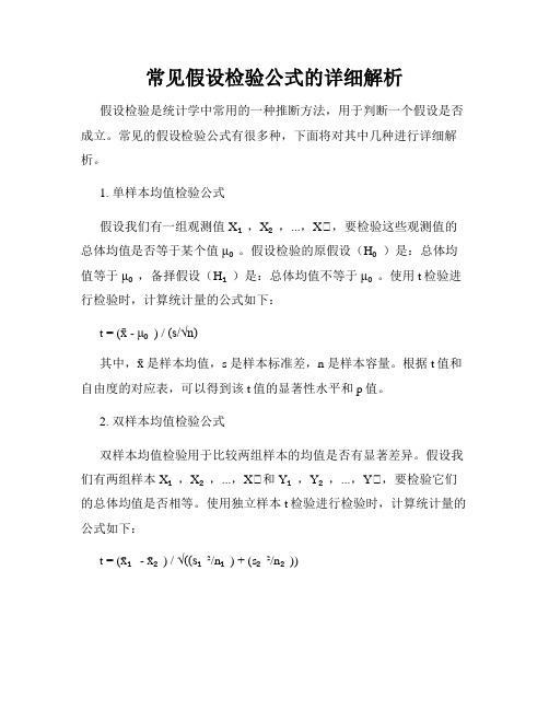
统计学假设检验类型公式整理在统计学中,假设检验是一种常用的方法,用于根据样本数据对总体特征进行推断。
通过假设检验,我们可以得出结论,判断某个总体参数是否符合我们的预期或者所提出的假设。
本文将整理常见的统计学假设检验类型及其相关公式,以帮助读者更好地理解和运用这些方法。
一、单样本均值检验单样本均值检验主要用于判断一个样本的平均值与已知总体的平均值是否有显著差异。
以下是单样本均值检验的公式:1. 步骤1:设定假设和显著性水平2. 步骤2:计算样本均值(x)和标准误差(SE)3. 步骤3:计算检验统计量(t值)4. 步骤4:计算p值5. 步骤5:作出决策,接受或拒绝原假设二、双样本均值检验双样本均值检验用于比较两个样本的均值是否存在显著差异。
以下是双样本均值检验的公式:1. 步骤1:设定假设和显著性水平2. 步骤2:计算两个样本的均值差值(x1 - x2)和标准误差(SE)3. 步骤3:计算检验统计量(t值)4. 步骤4:计算p值5. 步骤5:作出决策,接受或拒绝原假设三、配对样本均值检验配对样本均值检验用于比较同一组样本在不同时间或条件下的均值差异。
以下是配对样本均值检验的公式:1. 步骤1:设定假设和显著性水平2. 步骤2:计算配对样本的均值差值(d)和标准误差(SE)3. 步骤3:计算检验统计量(t值)4. 步骤4:计算p值5. 步骤5:作出决策,接受或拒绝原假设四、单样本比例检验单样本比例检验用于比较一个样本中某一属性的比例与已知总体比例是否有显著差异。
以下是单样本比例检验的公式:1. 步骤1:设定假设和显著性水平2. 步骤2:计算样本比例(p)和标准误差(SE)3. 步骤3:计算检验统计量(z值)4. 步骤4:计算p值5. 步骤5:作出决策,接受或拒绝原假设五、双样本比例检验双样本比例检验用于比较两个样本中某一属性的比例是否存在显著差异。
以下是双样本比例检验的公式:1. 步骤1:设定假设和显著性水平2. 步骤2:计算两个样本的比例差值(p1 - p2)和标准误差(SE)3. 步骤3:计算检验统计量(z值)4. 步骤4:计算p值5. 步骤5:作出决策,接受或拒绝原假设六、方差分析方差分析用于比较多个样本均值是否存在显著差异。
常见假设检验公式的详细解析
常见假设检验公式的详细解析假设检验是统计学中常用的一种推断方法,用于判断一个假设是否成立。
常见的假设检验公式有很多种,下面将对其中几种进行详细解析。
1. 单样本均值检验公式假设我们有一组观测值X₁,X₂,...,Xₙ,要检验这些观测值的总体均值是否等于某个值μ₀。
假设检验的原假设(H₀)是:总体均值等于μ₀,备择假设(H₁)是:总体均值不等于μ₀。
使用t检验进行检验时,计算统计量的公式如下:t = (x - μ₀) / (s/√n)其中,x是样本均值,s 是样本标准差,n 是样本容量。
根据t值和自由度的对应表,可以得到该t值的显著性水平和p值。
2. 双样本均值检验公式双样本均值检验用于比较两组样本的均值是否有显著差异。
假设我们有两组样本X₁,X₂,...,Xₙ和Y₁,Y₂,...,Yₙ,要检验它们的总体均值是否相等。
使用独立样本t检验进行检验时,计算统计量的公式如下:t = (x₁ - x₂) / √((s₁²/n₁) + (s₂²/n₂))其中,x₁和x₂分别是两组样本的均值,s₁和 s₂分别是两组样本的标准差,n₁和 n₂分别是两组样本的容量。
根据t值和自由度的对应表,可以得到该t值的显著性水平和p值。
3. 单样本比例检验公式单样本比例检验用于检验样本的比例是否等于某个给定的比例。
假设我们有一组观测值,成功的事件发生的次数为x,总事件发生的次数为n,要检验成功的概率是否等于某个给定的比例p₀。
使用正态分布的近似方法进行检验时,计算统计量的公式如下:z = (p - p₀) / √(p₀(1-p₀)/n)其中,p是样本成功的比例,p₀是给定的比例,n 是样本容量。
根据z值和显著性水平的对应关系,可以得到该z值的p值。
总结:上述所介绍的是常见假设检验公式中的几种,每种假设检验有其适用的前提条件和计算公式。
在进行假设检验时,需要注意选择适当的公式和假设检验方法,以及正确计算统计量并进行显著性检验。
CH11

思考与练习
7. 思考题 (1)Pearson积矩相关系数 经检验无统计学意义,是否 积矩相关系数r经检验无统计学意义 积矩相关系数 经检验无统计学意义, 意味着两变量间一定无关系? 意味着两变量间一定无关系? 答:对满足二元正态分布的随机样本,若直接计算 Pearson积矩相关系数且经检验无统计学意义,并不意味着 两变量间一定无关系,若两者之间是非线性关系的话,其 Pearson积矩相关系数也会无统计学意义,因此在确定两变 量间有无线性关系时应先绘出散点图进行直观考察后再作 出判断. (2)Pearson积矩相关系数 经检验有统计学意义,P值 积矩相关系数r经检验有统计学意义 积矩相关系数 经检验有统计学意义, 值 很小,是否意味着两变量间一定有很强的线性关系? 很小,是否意味着两变量间一定有很强的线性关系? 答:Pearson积矩相关系数r经检验有统计学意义,且P值 很小,并不意味着两变量间一定有很强的线性关系.参看 本章第一节线性相关应用中应注意的问题中的2,3,4,5 点.
χ2 χ2 +n
关于 Pearson 列联系数是否为零的检验等价于 Pearson χ 2 检验.
思考与练习
1.对某省 8 个地区水质的碘含量及其甲状腺肿的患病率作了调查后得到表 11-13 的数据,试问不同地区的甲状腺肿的患病率高低与本地区水质的碘含量有无关联?
假设检验(Hypothesis Testing)
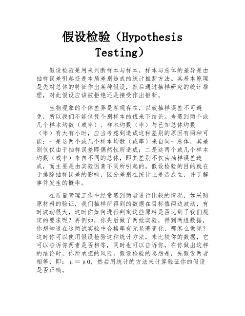
假设检验(HypothesisTesting)假设检验是用来判断样本与样本,样本与总体的差异是由抽样误差引起还是本质差别造成的统计推断方法。
其基本原理是先对总体的特征作出某种假设,然后通过抽样研究的统计推理,对此假设应该被拒绝还是接受作出推断。
生物现象的个体差异是客观存在,以致抽样误差不可避免,所以我们不能仅凭个别样本的值来下结论。
当遇到两个或几个样本均数(或率)、样本均数(率)与已知总体均数(率)有大有小时,应当考虑到造成这种差别的原因有两种可能:一是这两个或几个样本均数(或率)来自同一总体,其差别仅仅由于抽样误差即偶然性所造成;二是这两个或几个样本均数(或率)来自不同的总体,即其差别不仅由抽样误差造成,而主要是由实验因素不同所引起的。
假设检验的目的就在于排除抽样误差的影响,区分差别在统计上是否成立,并了解事件发生的概率。
在质量管理工作中经常遇到两者进行比较的情况,如采购原材料的验证,我们抽样所得到的数据在目标值两边波动,有时波动很大,这时你如何进行判定这些原料是否达到了我们规定的要求呢?再例如,你先后做了两批实验,得到两组数据,你想知道在这两试实验中合格率有无显著变化,那怎么做呢?这时你可以使用假设检验这种统计方法,来比较你的数据,它可以告诉你两者是否相等,同时也可以告诉你,在你做出这样的结论时,你所承担的风险。
假设检验的思想是,先假设两者相等,即:μ=μ0,然后用统计的方法来计算验证你的假设是否正确。
假设检验的基本思想1.小概率原理如果对总体的某种假设是真实的,那么不利于或不能支持这一假设的事件A(小概率事件)在一次试验中几乎不可能发生的;要是在一次试验中A竟然发生了,就有理由怀疑该假设的真实性,拒绝这一假设。
2.假设的形式H0——原假设,H1——备择假设双尾检验:H0:μ = μ0,单尾检验:,H1:μ < μ0,H1:μ > μ0假设检验就是根据样本观察结果对原假设(H0)进行检验,接受H0,就否定H1;拒绝H0,就接受H1。
Ch10假设检验(一个总体均值或比率)

• Alternative Hypotheses
– H1: Put here what is the challenge, the view of some characteristic of the population that, if it were true, would trigger some new action, some change in procedures that had previously defined “business as usual.”
© 2002 The Wadsworth Group
The Logic of Hypothesis Testing
• How will we decide?
– “In adjustment” means µ = 1.3250 minutes. – “Not in adjustment” means µ 1.3250 minutes.
• Which requires a change from business as usual? What triggers new action?
CHAPTER 10: Hypothesis Testing, One Population Mean or Proportion
to accompany
Introduction to Business Statistics
fourth edition, by Ronald M. Weiers
Presentation by Priscilla Chaffe-Stengel Donald N. Stengel
Nondirectional, Two-Tail Tests
H0: pop parameter = value H1: pop parameter value
生物统计学两个样本平均数假设检验

生物统计学两个样本平均数假设检验假设检验是一种基于样本数据来进行参数推断的统计方法,其基本思想是根据样本数据对总体参数进行估计,并根据估计结果进行参数假设的判断。
对于两个样本平均数的假设检验,通常分为独立样本和配对样本两种情况。
对于独立样本平均数假设检验,我们需要考虑两组样本来自于同一总体的情况。
首先,我们需要建立假设,通常分为零假设和备择假设。
零假设(H0)表示两个样本的平均数无显著差异,备择假设(H1)表示两个样本的平均数存在显著差异。
接下来,我们需要选择合适的统计检验方法。
当两个样本均为正态分布且方差已知时,可以使用Z检验;当两个样本均为正态分布但方差未知时,可以使用t检验;当两个样本均不服从正态分布时,可以使用非参数检验方法,如Wilcoxon秩和检验。
然后,我们需要计算检验统计量的值。
对于Z检验,检验统计量为差值的标准差除以差值的均值,再除以标准差的平方根。
对于t检验,检验统计量为差值的均值除以差值的标准差除以样本容量的平方根。
对于Wilcoxon秩和检验,检验统计量为两个样本的秩和之差。
最后,我们需要根据显著性水平来进行判断。
显著性水平是我们事先设定的,通常为0.05或0.01、我们可以计算出检验统计量对应的P值,P值表示在零假设成立的情况下,观察到样本数据或更极端情况出现的概率。
当P值小于显著性水平时,我们拒绝零假设,认为两组样本的平均数存在显著差异;当P值大于等于显著性水平时,我们接受零假设,认为两组样本的平均数无显著差异。
配对样本平均数假设检验是用于比较同一组样本在不同条件下的平均数是否存在显著差异。
其检验方法与独立样本平均数假设检验类似,只是在计算检验统计量时需要考虑两个样本之间的配对关系。
总之,两个样本平均数假设检验是生物统计学中常用的一种方法,通过对两组样本数据进行比较来判断它们的平均数是否存在显著差异。
我们需要建立适当的假设、选择合适的统计检验方法、计算检验统计量的值,并根据显著性水平来进行判断。
《双样本假设检验》课件

总结词
独立双样本t检验用于比较两个独立样本的 均值是否存在显著差异。
详细描述
独立双样本t检验的前提假设是两个样本相 互独立,且总体正态分布。通过计算t统计 量和自由度,可以判断两个样本均值是否存 在显著差异。
实例二:配对样本t检验
总结词
配对样本t检验用于比较同一观察对象在不同条件下的观测值是否存在显著差异 。
它通常包括以下步骤:提出假设、选择合适的统计量、确定显著性水平、进行统计推断、得出结论。
02
双样本假设检验的步骤
确定检验假设和备择假设
检验假设(H0)
用于确定两组样本均值是否相等的假设。
备择假设(H1)
与检验假设相对立的假设,即两组样本均值存在显著差异。
确定检验统计量
• 检验统计量是用于评估样本数据 与假设之间差异的统计量,常用 的有t检验、Z检验等。
双样本假设检验的重要性
在科学实验、医学研究、社会科学调 查等领域,双样本假设检验是一种非 常重要的统计工具。
VS
它可以帮助我们判断两组数据之间的 差异是否具有实际意义,从而为我们 的决策提供依据。
双样本假设检验的基本原理
双样本假设检验基于大数定律和中心极限定理,通过比较两组数据的差异来推断总体参数。
社会科学研究
调查研究
比较不同群体在某项调查指标上的差异,如性 别、年龄、教育程度等。
政策效果评估
比较政策实施前后的效果,评估政策的有效性 。
行为研究
分析不同情境下个体行为的差异,解释行为背后的原因。
质量控制和生产过程控制
质量控制
检测产品或服务的质量是否符合标准或客户 要求。
过程能力分析
评估生产过程的能力水平,识别过程改进的 潜力。
- 1、下载文档前请自行甄别文档内容的完整性,平台不提供额外的编辑、内容补充、找答案等附加服务。
- 2、"仅部分预览"的文档,不可在线预览部分如存在完整性等问题,可反馈申请退款(可完整预览的文档不适用该条件!)。
- 3、如文档侵犯您的权益,请联系客服反馈,我们会尽快为您处理(人工客服工作时间:9:00-18:30)。
© 2002 The Wadsworth Group
Chapter 11 - Key Terms
Independent vs Dependent Samples
• Independent Samples:
Samples taken from two different populations, where the selection process for one sample is independent of the selection process for the other sample.
© 2002 The Wadsworth Group
Test of (µ1 – µ2), Unequal Variances, Independent Samples
• Test Statistic
t = ( x1 x 2 ) ( m 1 m 2 ) 0 s1
2
+
2 1
s2
2
n1 where df =
• Dependent Samples:
– Testing the relative fuel efficiency of 10 trucks that run the same route twice, once with the current air filter installed and once with the new filter.
© 2002 The Wadsworth Group
Test of (µ1 – µ2), s1 = s2, Populations Normal
• Test Statistic
[x – x ] – [m – m ] t = 1 2 1 2 0 ÷ 2 1 + 1 ÷ sp n n ÷ ÷ 1 2÷ (n –1)×2 + (n –1)× 2 s s 1 2 2 where s p2 = 1 n +n – 2 1 2 and df = n1 + n2 – 2
– difference of two population means – difference of two population proportions
• Matched, or paired, observations • Average difference
© 2002 The Wadsworth Group
• II. Rejection Region
a = 0.05 df = 25 + 25 – 2 = 48 Reject H0 if t > 2.011 or t < –2.011
R e je c t H
0
D o N ot R e je c t H
R e je c t H
0
0
t= -2 .0 1 1
© 2002 The Wadsworth Group
Examples: Independent versus Dependent Samples
• Independent Samples:
– Testing a company’s claim that its peanut butter contains less fat than that produced by a competitor.
© 2002 The Wadsworth Group
Ask the following questions:
Identifying the Appropriate Test Statistic
• Are the data from measurements (continuous variables) or counts (discrete variables)? • Are the data from independent samples? • Are the population variances approximately equal? • Are the populations approximately normally distributed? • What are the sample sizes?
n2 n1 ) + ( s 2 n 2 )
2 2 2
( s
2
( s1 n1 ) n1 1
+
( s2 n2 ) n2 1
2
2
© 2002 The Wadsworth Group
Example, Unequal-Variances t-Test, Independent Samples
• Suppose analysis of two independent samples from normally distributed populations reveal the following values:
Since the test statistic of t = – 1.289 falls between the critical bounds of t = ± 2.011, we do not reject the null hypothesis with at least 95% confidence.
CHAPTER 11: Hypothesis Testing Involving Two Sample Means or Proportions
to accompany
Introduction to Business Statistics
fourth edition, by Ronald M. Weiers
t= 2 .0 1 1
© 2002 The Wadsworth Group
t-Test, Problem 11.2 cont.
• III. Test Statistic
24× .8)2 + 24×.1)2 = 1460.16 + 1564.64 = 63.225 (8 s p2 = (7 25 + 25 – 2 48 t= x –x 1 2 s p2 1 + 1 n n 1 2
÷ ÷ ÷ ÷ ÷ ÷
=
77.1– 80.0 = –1.289 1 1 ÷ 63.225 + ÷ 25 25 ÷
© 2002 The Wadsworth Group
t-Test, Problem 11.2 cont.
• IV. Conclusion:
Presentation by Priscilla Chaffe-Stengel Donald N. Stengel
© 2002 The Wadsworth Group
Chapter 11 - Learning Objectives
• Select and use the appropriate hypothesis test in comparing
© 2002 The Wadsworth Group
t-Test, Two Independent Means
• I. H0: µ1 – µ2 = 0 H1: µ1 – µ2 0
The two videotapes are equally effective. There is no difference in student performance. The two videotapes are not equally effective. There is a difference in student performance.
– – – – Means of two independent samples Means of two dependent samples Proportions of two independent samples Variances of two independent samples
• Construct and interpret the appropriate confidence interval for differences in
© 2002 The Wadsworth Group
Example, Calculation of the Degrees of Freedom for the t-Test
• Dependent Samples:
Samples taken from two populations where either (1) the element sampled is a member of both populations or (2) the element sampled in the second population is selected because it is similar on all other characteristics, or “matched,” to the element selected from the first population
• V. Implications:
There is not enough evidence for us to conclude that one videotape training session is more effective than the other.
• p-value:
Using Microsoft Excel, type in a cell: =TDIST(1.289,48,2) The answer: p-value = 0.203576