Interactive Terascale Particle Visualization
粒子特效参数的设置一粒子软件particleIllusion系列教程
粒子特效参数的设置一粒子软件particleIllusion系列教程粒子特效参数的设置一粒子软件particleIllusion系列教程Emitter 與 Particles 的關係在 illusion 中我們會選擇 Emitter﹙噴射體﹚來製造效果,illusion 為方便使用者,每個Emitter都由1個或更多Particle﹙分子﹚所組成。
我們可以替Emitter 下一定義:「Emitter 是由1個或更多Particle所組合而成」。
Emitter 有參數可調整,每一個 Particle 也有參數可調整,這兩者有什麼差異。
Particle 參數定義:「調整分子的特徵」。
Emitter 參數定義:「調整 Particle﹙分子﹚參數的設定」。
大家可能會搞混,沒關係接下來以實例說明。
Emitter/Weight步驟1:請先在「舞台視窗」加一Emitter "Green-Yellow"﹙圖 1﹚,按「Play」播放。
圖 1:加入 Emitter步驟 2:在第「61」格可見到﹙圖 2﹚的狀況,Emitter 是「四面八方」噴出。
圖 2:Emitter 效果步驟 3:將現在格數設為「1」,然後調整 Emitter 的 Weight 參數﹙圖3 的"B"﹚,我們會發覺怎麼調整都沒有效果,這是因為Particle/Weight 設成"0"。
圖 3:Emitter/Weight 的參數Particle/Weight再回溯文章開頭,Emitter 參數定義:「調整Particle﹙分子﹚參數的設定」,所以真正控制權還是在 Particle 的參數。
展開 Emitter 下的 Particle "colorful",當 Particle/Weight 設成"0" 時﹙圖 4﹚,在 Emitter/Weight 如何調整都沒有用。
AE中particular插件中英文对照

AE中particular插件中英文对照(一)Emitter(发射器)Particular/sec(粒子/秒)——每秒钟发射粒子的数量。
EmitterType(发射器类型)——它决定发射粒子的区域和位置。
Point(点)——从一点发射出粒子Box(盒子)——粒子会从立体盒子中发射出来,(EmitterSize中XYZ是指发射器大小)Sphere(球形)——和Box很像,只不过发射区域是球形Grid(网格)——(在图层中虚拟网格)从网格的交叉点发射粒子Light(灯光)——(要先新建一个LightLayer)几个LightLayer可以共用一个Particular。
Layer——使用合成中的3D图层生成粒子,LayerGrid——同上,发射器从图层网格发射粒子,像Grid一样。
Direction(方向)Uniform(统一)——任一粒子发射类型发射粒子时,会向各个方向移动。
Directional(特定方向)——(如枪口喷射)通过调节X、Y、ZRotation来实现。
Bi-Directional(相反特定方向)——和Directional十分相似,但是向着两个完全相反的方向发射。
通常为180度。
Disc(盘状)——通常只在两个维度上,形成一个盘形。
Outwards(远离中心)——粒子会始终向远离发射点的方向移动。
而Uniform是随机的。
DirectionSpread(方向拓展)——可以控制粒子发射方向的区域。
粒子会向整个区域的百分之几运动。
(即粒子发射方向有多宽)Velocity(速度)——粒子每秒钟运动的像素数。
VelocityRandom——每个粒子Velocity的随机性会随机增加或者减小每个粒子的Velocity。
VelocityDistribution()——VelocityfromMotion(速度跟随运动)——粒子在向外运动的同时也会跟随发射器的运动方向运动。
LayerEmitter(图层发射器)Layer(选用哪一个图层作为发射器)LayerSampling()——2CurrentTime(当前时间)ParticularBirthTime(粒子生成时间)LayerRGBUsage(图层颜色使用方式)Lightness-Size——随着图像的明暗变化,粒子的大小也跟着变化Lightness-Velocity——随着图像的明暗变化,粒子的速度也跟着变化Lightness-Rotation——随着图像的明暗变化,粒子的旋转也跟着变化RGB-Size,Vel,Rot——随着图像的颜色变化,粒子的大小,速度,旋转同时变化RGB-ParticleColor——随着图像的颜色变化,粒子的颜色也跟着变化GridEmitter(网格发射器)ParticularinX(粒子在X方向上的数量)ParticularinY(粒子在Y方向上的数量)ParticularinZ(粒子在Z方向上的数量)Type(类型)PeriodicBurst(周期性爆炸)——粒子同时发射出来Traverse(横渡)——粒子以行的形式依次发射出来EmissionExtrasPreRun(提前运行)PerodicityRndRandomSeed(随机性)——随即数值的开始点,它一变整个插件的随机性都会变化Particle(粒子)Life[sec]——实际上就是粒子生存的时间。
AE粒子流教程 实现流动的粒子效果
AE粒子流教程:实现流动的粒子效果在AE软件中,粒子效果是非常常见且常用的特效之一。
它能够通过模拟出各种粒子的运动和交互,创造出各种惊艳的效果,使得视频更加生动和有趣。
在本教程中,我们将学习如何实现流动的粒子效果。
首先,打开AE软件并创建一个新的合成。
选择你想要使用的画布大小和帧速率,并创建一个空白的合成。
接下来,我们需要创建粒子系统。
点击“Layer”菜单,选择“New”并选择“Solid”选项。
设置合适的尺寸和颜色,然后点击“OK”按钮。
然后,在合成中右键单击这个新创建的图层,选择“Effect”和“Simulation”菜单。
在下拉菜单中,选择“CC Particle Systems II”。
这将在图层上应用一个默认的粒子系统效果。
现在,我们需要调整粒子系统的参数,使得效果更具流动性。
在AE界面右侧的“Effects Controls”窗口中,可以看到“Particle”选项。
展开这个选项,我们可以看到一系列参数。
首先,调整“Particle Type”参数。
选择“Line”的选项,这将使得粒子呈现为线条状。
如果你想要更细的线条,可以调整“Birth Size”和“Death Size”参数。
接下来,调整“Particle Life”参数。
增加这个数值将使得粒子的寿命更长,从而使得流动效果更加明显。
然后,我们需要给粒子添加运动效果。
在“Physics”选项中,调整“Velocity”和“Gravity”参数。
增加“Velocity”值将使得粒子运动速度更快,而增加“Gravity”值将使得粒子受到更大的重力影响。
此外,你还可以调整其他参数,如“Opacity over Life”,“Size over Life”和“Color over Life”,以使得粒子的外观和变化更加多样化。
现在,我们已经完成了流动的粒子效果的制作。
你可以通过按下空格键预览效果,并根据需要进行微调。
如果你想要更加个性化的流动粒子效果,你可以尝试添加其他图层,如文字、形状或者图片。
AE常用particular粒子中英文对照表讲解
AE常用particular粒子中英文对照表讲解为什么particular是个粒子生成器?在particular中粒子有好几种类型。
1.粒子可以是particular自己生成的一张图像。
球星、发光球体、星状、云状、烟状。
2.当我们使用Custom Particular(定制粒子)时,意味着我们可以使用任何图像作为粒子。
所以什么是Particular?Particular就是图像。
Particular Generater(粒子生成器)是用来生成和控制粒子的工具。
控制各种特性,例如速度、方向、大小和颜色、以及物理属性,如重力turbulence(涡流)等等。
Particular界面(默认设置)Emitter(发射器)Particular/sec (粒子数量/秒)—100—每秒钟发射粒子的数量。
Emitter Type(发射器类型)——它决定发射粒子的区域和位置。
Point(点)——从一点发射出粒子Box(盒子)——粒子会从立体盒子中发射出来,(Emitter Size 中XYZ是指发射器大小)Sphere(球体)——和Box很像,只不过发射区域是球形Grid(网格)——(在图层中虚拟网格)从网格的交叉点发射粒子Light(灯光)——(要先新建一个Light Layer)几个Light Layer可以共用一个Particular。
Layer(图层)——使用合成中的3D图层生成粒子,Layer Grid(图层网格)——同上,发射器从图层网格发射粒子,像Grid(网格)一样。
Position位置XYPosition位置Z 0Position Subframe位置子帧Linear(线性)10xLinear(10x线性)10x Smooth(10x平滑)Exact(slow)精确(慢)Direction(方向)Uniform(统一)——任一粒子发射类型发射粒子时,会向各个方向移动。
Directional(方向)——(如枪口喷射)通过调节X、Y、Z Rotation来实现。
particle metrix使用步骤-概述说明以及解释
particle metrix使用步骤-概述说明以及解释1.引言1.1 概述Particle Metrix是一款用于颗粒分析的软件工具,具有简单易用的界面和强大的数据处理功能。
该软件可以帮助科研人员快速准确地分析样品中的颗粒体积分布、颗粒大小和形状等关键参数,为科研实验和工程项目提供可靠的数据支持。
本文将介绍Particle Metrix的使用步骤,旨在帮助读者快速掌握该软件的操作方法,并有效地提高数据处理的效率和准确性。
通过学习本文内容,读者可以更好地应用Particle Metrix进行颗粒分析,并探索其在不同领域的应用前景。
1.2 文章结构本文共分为三部分:引言、正文和结论。
在引言部分,将首先对Particle Metrix进行简要介绍,然后说明本文的结构和目的。
在正文部分,将详细介绍Particle Metrix的相关信息,包括其功能、使用步骤和数据分析方法。
在结论部分,将对文章进行总结,探讨Particle Metrix的应用前景,并展望未来可能的发展方向。
1.3 目的本文旨在向读者介绍Particle Metrix的使用步骤,帮助用户更好地了解和掌握这一技术工具。
通过详细的步骤说明和实际操作示例,读者将能够快速上手并利用Particle Metrix进行粒子分析和数据处理。
同时,本文也旨在展示Particle Metrix在科学研究和工程应用中的潜在价值和应用前景,希望能够为读者提供参考和启发,推动该领域的进步和发展。
2.正文2.1 Particle Metrix简介Particle Metrix是一款专业的颗粒分析软件,主要用于对颗粒或微粒的形状、大小和分布进行分析。
该软件能够快速、准确地获取微观颗粒的相关数据,为科研和工程领域提供了重要的分析工具。
Particle Metrix具有直观的操作界面和强大的数据处理能力,用户可以通过简单的操作即可完成颗粒分析过程。
该软件支持多种数据格式的导入和导出,方便用户与其他分析工具进行数据交换。
particular参数详解

particular参数详解1.Emitter面板粒子发生器:用于产生粒子,并设定粒子的大小、形状、类型、初始速度与方向等属性。
1.1 Particles/sec控制每秒钟产生的粒子数量,该选项可以通过设定关键帧设定来实现在不同的时间内产生的粒子数量。
1.2 Emitter Type设定粒子的类型。
粒子类型主要有point、box、sphere、grid、light、layer、layer grid等七种类型。
1.3 Position XY & Position Z设定产生粒子的三维空间坐标。
(可以设定关键帧)1.4 Direction用于控制粒子的运动方向。
1.5 Direction Spread控制粒子束的发散程度,适用于当粒子束的方向设定为Directional、Bi-directional、Disc和Outwards等四种类型。
对于粒子束方向设定为Uniform和以灯光作为粒子发生器等情况时不起作用。
1.6 X,Y and Z Rotation用于控制粒子发生器的方向。
1.7 Velocity用于设定新产生粒子的初始速度。
1.8 Velocity Random默认情况下,新产生的粒子的初速度是相等的,我们可以通过该选项为新产生的粒子设定随机的初始速度。
1.9 Velocity from Motion让粒子继承粒子发生器的速度。
此参数只有在粒子发生器是运动的情况下才会起作用。
该参数设定为负值时能产生粒子从粒子发生器时喷射出来一样的效果。
设定为正值时,会出现粒子发生器好象被粒子带着运动一样的效果。
当该参数值为0时,没有任何效果。
1.10 Emitter Size X,Y and Z当粒子发生器选择Box, Sphere, Grid and Light时,设定粒子发生器的大小。
对于Layer and Layer Grid粒子发生器,只能设定Z参数。
2.Particle面板在particle参数组可以设定粒子的所有外在属性,如大小、透明度、颜色,以及在整个生命周期内这些属性的变化。
ParticleIllusion基础教程l
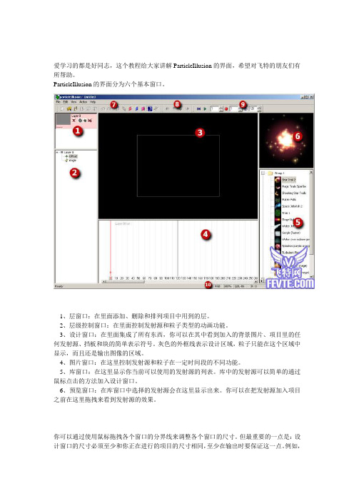
爱学习的都是好同志,这个教程给大家讲解ParticleIllusion的界面,希望对飞特的朋友们有所帮助。
ParticleIllusion的界面分为六个基本窗口。
1、层窗口:在里面添加、删除和排列项目中用到的层。
2、层级控制窗口:在里面控制发射源和粒子类型的动画功能。
3、设计窗口:在里面集成了所有东西,你可以在其中看到加入的背景图片、项目里的任何发射源、挡板和块的简单表示符号。
灰色的外框线表示设计区域,粒子只能在这个区域中显示,而且还是输出图像的区域。
4、图片窗口:在这里控制发射源和粒子在一定时间段的不同功能。
5、库窗口:在这里显示你当前可以使用的发射源的列表。
库中的发射源可以简单的通过鼠标点击的方法加入设计窗口。
6、预览窗口:在库窗口中选择的发射源会在这里显示出来。
你可以在把发射源加入项目之前在这里拖拽来看到发射源的效果。
你可以通过使用鼠标拖拽各个窗口的分界线来调整各个窗口的尺寸。
但最重要的一点是:设计窗口的尺寸必须至少和你正在进行的项目的尺寸相同,至少在输出时要保证这一点。
例如,如果你正在做一个640*480的项目,设计窗口就至少要有640*480大小,否则你就得不到全尺寸的输出图片。
在Illusion里你还需要学习许多其他的对话框和鼠标操作。
和其他教程中对每一项功能详细里表说明不同,我认为通过在一个例子中逐步讲解每一项功能会更合适一些。
通过对下面一些例子的学习你将会慢慢了解Illusion的使用。
Illusion 教程第一讲:简介Illusion是一个富有创造性的后期处理软件,可以帮助你极大的提高你的图像制作工作。
要求平台:Win95,Win98,WinNT(或更高)机器配置:至少32M内存,你的显卡在800*600分辨率下至少16位色(建议24或者32位色),这个配置对于大多数用户来说应该不成问题。
Illusion支持OpenGL硬件加速,所以如果你的显卡支持OpenGL的话,将会加快图像处理速度。
AE之particular插件英汉对照

Particular(AE)插件为什么particular是个粒子生成器?在particular中粒子有好几种类型。
1.粒子可以是particular自己生成的一张图像。
球星、发光球体、星状、云状、烟状。
2.当我们使用Custom Particular(定制粒子)时,意味着我们可以使用任何图像作为粒子。
所以什么是Particular?Particular就是图像。
Particular Generater(粒子生成器)是用来生成和控制粒子的工具。
控制各种特性,例如速度、方向、大小和颜色、以及物理属性,如重力turbulence(涡流)等等。
Particular界面Emitter(发射器)Particular/sec(粒子/秒)——每秒钟发射粒子的数量。
Emitter Type(发射器类型)——它决定发射粒子的区域和位置。
Point(点)——从一点发射出粒子Box(盒子)——粒子会从立体盒子中发射出来,(Emitter Size中XYZ是指发射器大小)Sphere(球形)——和Box很像,只不过发射区域是球形Grid(网格)——(在图层中虚拟网格)从网格的交叉点发射粒子Light(灯光)——(要先新建一个Light Layer)几个Light Layer可以共用一个Particular。
Layer——使用合成中的3D图层生成粒子,Layer Grid——同上,发射器从图层网格发射粒子,像Grid一样。
Direction(方向)Uniform(统一)——任一粒子发射类型发射粒子时,会向各个方向移动。
Directional(特定方向)——(如枪口喷射)通过调节X、Y、Z Rotation来实现。
Bi-Directional(相反特定方向)——和Directional十分相似,但是向着两个完全相反的方向发射。
通常为180度。
Disc(盘状)——通常只在两个维度上,形成一个盘形。
Outwards(远离中心)——粒子会始终向远离发射点的方向移动。
AE常用particular粒子中英文对照表
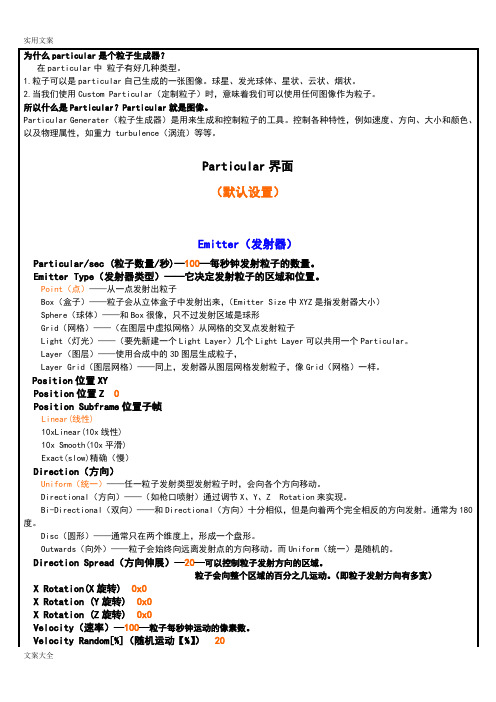
Particular界面
(默认设置)
Emitter(发射器)
Particular/sec (粒子数量/秒)—100—每秒钟发射粒子的数量。
RGB-Particle Color(RGB-粒子颜色)——随着图像的颜色变化,粒子的颜色也跟着变化
None无
Grid Emitter(网格发射)----在(网格、图层网格下有效)
Particular in X(粒子在X方向上的数量)5
Particular in Y(粒子在Y方向上的数量)5
Particular in Z(粒子在Z方向上的数量)1
Start at Birth-Loop(出生时开始循环演示)---从开始采样直到最后不断循环。
Start at Birth-Stretch(出生时开始伸展演示)---从开始采样一次延长到结束。
Random-Still Frame(随机-静帧)
Random-Play Once(随机-演示一遍)
Random-Loop(随机-循环演示)
Velocity Distribution(速度分布)—0.5—
Velocity from Motion[%](继承运动速度【%】)20
——粒子在向外运动的同时也会跟随发射器的运动方向运动。
Emitter Size X(发射器尺寸X )50
Emitter Size Y (发射器尺寸Y )50
Emitter Size Z (发射器尺寸Z)50
Size Random[%](尺寸随机【%】)—0—增加粒子大小的随机性
AE常用particular粒子中英文对照表

At Birth(颜色)—白—设置粒子出生时的颜色
Color Random[%](颜色随机【%】)—0—随机改变色相
Color over Life(生命期颜色)——颜色随时间变化,图形表示;
Transfer Mode(应用模式)——控制当粒子重叠时颜色的混合方式
Particle(粒子)
Life[sec](生命/秒)—3—实际上就是粒子生存的时间。
Life Random[%](生命随机【%】)—0—随机增加或者减少粒子的生命
Particle Type(粒子类型)
Sphere(球体)——是使用2D的球形图片作为粒子
Glow Sphere(发光球体)——同上,粒子加强型。NO DOF意思是这些粒子没有景深效果
Start at Birth-Loop(出生时开始循环演示)---从开始采样直到最后不断循环。
Start at Birth-Stretch(出生时开始伸展演示)---从开始采样一次延长到结束。
Random-Still Frame(随机-静帧)
Random-Play Once(随机-演示一遍)
Random-Loop(随机-循环演示)
Shadowlet for Aux(补充阴影)—off关—子粒子阴影开关;
Shadowlet Settings阴影设置
Color颜色
Color Strength颜色强度100
Opacity不透明度5
Adjust Size校正大小100
Adjust Distance校正距离100
Placement方位Auto自动
Bi-Directional(双向)——和Directional(方向)十分相似,但是向着两个完全相反的方向发射。通常为180度。
ae particular 中英文对照表
AE particular 中英文对照表一、介绍AE particular是一款常用的AE插件,它提供了丰富的粒子效果和发射器的功能,可以帮助用户快速制作出惊艳的特效动画。
在使用AE particular插件的过程中,往往需要对一些参数进行调整,而很多用户可能对这些参数的中英文对照不是很熟悉。
本文就是总结了AE particular插件中常用参数的中英文对照表,希望能够帮助到大家。
二、中英文对照表1. 粒子系统 - Particle System2. 发射器 - Emitter3. 粒子类型 - Particle Type4. 形状 - Shape5. 大小 - Size6. 速度 - Speed7. 旋转 - Rotation8. 颜色 - Color9. 透明度 - Opacity10. 弹力 - Bounce11. 生命周期 - Life12. 粒子数量 - Particle Count13. 粒子间距 - Particle Distance14. 发射角度 - Emit Angle15. 散布角度 - Spread Angle三、注意事项在使用AE particular插件时,一定要根据具体的需求来调整参数,以达到最好的效果。
也要注意插件的版本是否与AE软件版本兼容,避免出现不必要的问题。
总结:以上就是AE particular中常用参数的中英文对照表,希望能够给大家在使用AE particular插件时带来一些方便。
希望大家都能够在动画制作的道路上不断进步,创作出更加精彩的作品。
AE particular作为一款专业的AE插件,其强大的功能和灵活的特效调节,能够在制作特效动画时发挥出非常重要的作用。
由于AE particular插件拥有众多的参数和选项,许多用户在使用过程中可能会遇到一些困惑。
下面将继续为大家介绍AE particular插件中更多常用参数的中英文对照表,以及一些参数的功能和调节方法。
AE常用particular粒子中英文对照表

Point(点)——从一点发射出粒子
Box(盒子)——粒子会从立体盒子中发射出来,(Emitter Size中XYZ是指发射器大小)
Sphere(球体)——和Box很像,只不过发射区域是球形
Grid(网格)——(在图层中虚拟网格)从网格的交叉点发射粒子
粒子会向整个区域的百分之几运动。(即粒子发射方向有多宽)
X Rotation(X旋转)0x0
X Rotation (Y旋转)0x0
X Rotation (Z旋转)0x0
Velocity(速率)—100—粒子每秒钟运动的像素数。
Velocity Random[%](随机运动【%】)20
——每个粒子Velocity的随机性会随机增加或者减小每个粒子的Velocity。
Split Clip-Play Once(分段-演示一遍)
Split Clip-Loop(分段-循环演示)
Split Clip-Stretch(分段-伸展演示)——把定制粒子分离开。
Current Frame-Freeze(当前帧-冻结)
Random Seed(随机种子)1
Number of Clips(分段数量)—2—分离的个数—将粒子分成几份
Velocity Distribution(速度分布)—0.5—
Velocity from Motion[%](继承运动速度【%】)20
——粒子在向外运动的同时也会跟随发射器的运动方向运动。
Emitter Size X(发射器尺寸X )50
Emitter Size Y (发射器尺寸Y )50
Emitter Size Z (发射器尺寸Z)50
AE常用particular粒子中英文对照表

Particular界面
(默认设置)
Emitter(发射器)
Particular/sec (粒子数量/秒)—100—每秒钟发射粒子的数量。
Velocity Distribution(速度分布)—0.5—
Velocity from Motion[%](继承运动速度【%】)20
——粒子在向外运动的同时也会跟随发射器的运动方向运动。
Emitter Size X(发射器尺寸X )50
Emitter Size Y (发射器尺寸Y )50
Emitter Size Z (发射器尺寸Z)50
Glow(辉光)
Size尺寸300
Opacity不透明度25
Feather羽化100
Transfer Mode(应用模式)——Glow与粒子的叠加模式
Normal普通
Add相加
Screen屏幕
Streaklet(条纹)——条状痕
Random Seed(随机种子)
No Streaks(无条纹)—7—条痕数,条状痕由几个粒子组成
粒子会向整个区域的百分之几运动。(即粒子发射方向有多宽)
X Rotation(X旋转)0x0
X Rotation (Y旋转)0x0
X Rotation (Z旋转)0x0
Velocity(速率)—100—粒子每秒钟运动的像素数。
Velocity Random[%](随机运动【%】)20
——每个粒子Velocity的随机性会随机增加或者减小每个粒子的Velocity。
AE常用particular粒子中英文对照表

在particular中粒子有好几种类型。
1.粒子可以是particular自己生成的一图像。
球星、发光球体、星状、云状、烟状。
2•当我们使用Custom Particular (定制粒子)时,意味着我们可以使用任何图像作为粒子。
所以什么是Particular ?Particular就是图像。
Particular Gen erater (粒子生成器)是用来生成和控制粒子的工具。
控制各种特性,例如速度、方向、大小和颜色、以及物理属性,如重力turbulenee (涡流)等等。
Particular 界面(默认设置)Emitter (发射器)Particular/sec (粒子数量/秒)—100—每秒钟发射粒子的数量。
Emitter Type (发射器类型)--- 它决定发射粒子的区域和位置。
Point (点)一一从一点发射出粒子Box (盒子)一一粒子会从立体盒子中发射出来,(Emitter Size中XYZ是指发射器大小)Sphere (球体)一一和Box很像,只不过发射区域是球形Grid (网格)——(在图层中虚拟网格)从网格的交叉点发射粒子Light (灯光)--- (要先新建一个Light Layer)几个Light Layer 可以共用一个Particular。
Layer (图层)一一使用合成中的3D图层生成粒子,Layer Grid (图层网格)--- 同上,发射器从图层网格发射粒子,像Grid (网格)一样。
Position 位置XYPosition 位置Z 0Position Subframe 位置子帧Linear(线性)10xLinear(10x 线性)10x Smooth(10x 平滑)Exact(slow)精确(慢)Direction (方向)Un iform (统一)一一任一粒子发射类型发射粒子时,会向各个方向移动。
Directional (方向)一一(如枪口喷射)通过调节X、Y、Z Rotation来实现。
AE中如何制作虚幻粒子效果
AE中如何制作虚幻粒子效果在Adobe After Effects(AE)软件中,我们可以通过使用粒子系统来创建各种令人惊叹的视觉效果。
其中一种令人难以置信的效果是虚幻粒子效果。
虚幻粒子效果可以创建出逼真的粒子效果,使画面看起来非常炫酷。
下面是一个简单的教程,将指导您如何在AE中制作虚幻粒子效果。
第一步是打开AE软件并创建一个新的合成。
点击“文件”然后选择“新建合成”。
输入所需的合成尺寸和持续时间,然后点击“确定”。
接下来,在合成中创建一个新的“固态”图层。
点击“图层”然后选择“新建”然后“固态”。
这将创建一个空的图层。
选择“固态”图层后,点击“效果”然后选择“模拟效果”和“粒子系统II”。
这将在图层上应用粒子系统效果。
在粒子系统设置中,你可以调整各种参数来创建所需的虚幻粒子效果。
首先要调整的是“发射器”选项。
在“发射器”下的“发射器类型”中,选择“散射”。
在“散射”下,你可以调整粒子的数量,速度和角度等。
增加粒子的数量会让效果更加密集,增加速度会让粒子运动更快,调整角度会改变粒子的发射角度。
下一个要调整的是“粒子”选项。
在这里,你可以改变粒子的大小、生命周期和透明度等。
增加粒子的大小会让它们更加明显,调整生命周期会改变粒子的持续时间,调整透明度会使粒子出现或消失的方式变得更加渐进。
在虚幻粒子效果中,粒子的颜色选择非常重要。
你可以在“颜色下”部分调整粒子的颜色设置。
通过调整颜色的亮度、饱和度和透明度,你可以创建出不同的虚幻效果。
除了基本的粒子设置之外,你还可以尝试调整“物理”选项来改变粒子的行为。
例如,你可以添加引力或风力等外力来调整粒子的飘动效果。
当你完成了所有的设置后,可以点击播放按钮预览你的虚幻粒子效果。
如果不满意,可以继续调整参数直到达到理想的效果。
最后,点击“合成”然后选择“添加合成到渲染队列”来渲染你的合成。
选择所需的输出设置,然后点击“渲染”。
通过编写此简单教程,我们了解到了在AE中制作虚幻粒子效果的基本步骤。
particleIllusion 使用快速入门
快顯清單:在Windows的系統中,按下滑鼠右鍵可出現的選單。
Keyframe:關鍵畫格或關鍵影格,這是定義一整段動畫時,僅針對部分的畫格進行設定,而這些特定的畫格,就稱為Keyframe。在particleIllusion主要是用在Key-Position (關鍵位置),主要是紀錄運動的位置,概念上與Keyframe是相同的。
以下的畫面截圖,使用particleIllusion 3.0 Windows版本,在Mac版本上使用相同,Mac與Windows的particleIllusion 3.0試用版亦同。
幾個基本的概念
emitter:發射器
frame:畫格、影隔,這是particleIllusion的長度單位。NTSC的影視系統,每秒30個畫格;PAL的影視系統,每秒25個畫格;FILM (電影)的系統,每秒24個畫格。
點選以下的圖片,可在新視窗開啟較大的圖片。
點選以下的圖片,可在新視窗開啟較大的圖片。
點選以下的圖片,可在新視窗開啟較大的圖片。
點選以下的圖片,可在Байду номын сангаас視窗開啟較大的圖片。
點選以下的圖片,可在新視窗開啟較大的圖片。
1‧我要發表意見
資料整理:仕冶資訊技術服務小組
particleillusionqtcreator快速入门吉他快速入门lol快速入门dota2快速入门单反使用入门java快速入门ps快速入门photoshop快速入门php快速入门
particleIllusion使用快速入門
作者:楊繼華
Page:1-1
資料整理:仕冶資訊技術服務小組
本快速入門教學,說明入門使用者必須最先了解的工具與位置。
- 1、下载文档前请自行甄别文档内容的完整性,平台不提供额外的编辑、内容补充、找答案等附加服务。
- 2、"仅部分预览"的文档,不可在线预览部分如存在完整性等问题,可反馈申请退款(可完整预览的文档不适用该条件!)。
- 3、如文档侵犯您的权益,请联系客服反馈,我们会尽快为您处理(人工客服工作时间:9:00-18:30)。
Interactive Terascale Particle VisualizationDavid Ellsworth ∗Advanced Management Technology,Inc.NASA Ames Research CenterBryan Green †Advanced Management Technology,Inc.NASA Ames Research CenterPatrick Moran ‡NASA Ames ResearchCenterFigure 1:Streakline visualization of a 2TB turbopump data set,with particles colored by pressure.Because the geometry is proprietary,the pump blades are not shown and some remaining geometry is decimated.A BSTRACTThis paper describes the methods used to produce an interactive vi-sualization of a 2TB computational fluid dynamics (CFD)data set using particle tracing (streaklines).We use the method introduced by Bruckschen et al.[3]that precomputes a large number of parti-cles,stores them on disk using a space-filling curve ordering that minimizes seeks,then retrieves and displays the particles according to the user’s command.We describe how the particle computation can be performed using a PC cluster,how the algorithm can be adapted to work with a multi-block curvilinear mesh,how scalars can be extracted and used to color the particles,and how the out-of-core visualization can be scaled to 293billion particles while still achieving interactive performance on PC pared to the earlier work,our data set size and total number of particles are an order of magnitude larger.We also describe a new compression technique that losslessly reduces the amount of particle storage by 41%and speeds the particle retrieval by about 20%.CR Categories:I.3.8[Computer Graphics]:Applications;E.4[Coding and Information Theory]:Data compaction and compression; D.1.3[Programming Techniques]:Concurrent Programming—Parallel programming∗e-mail:ellswort@ †e-mail:bgreen@‡e-mail:patrick.j.moran@Keywords:visualization,particle tracing,large data,out-of-core,PC hardware,clusters,computational fluid dynamics.1I NTRODUCTIONInteractive visualization of data sets containing a terabyte or more is difficult to do even on the largest systems.Very few systems have enough memory to hold the data in memory.Out-of-core vi-sualization using traditional visualization algorithms is impossible since the data rates of tens of gigabytes per second necessary can-not currently be achieved.However,it is currently quite possible to generate multi-terabyte data sets of CFD or physics calculations on today’s supercomputers.In addition,using PC-class hardware for the visualization is desirable since this allows scientists to examine their results on their desktop.One approach that scales to large data sets is to precompute the visualization.In most cases,the resulting geometry can be dis-played interactively.For time-varying data,a visualization can be computed for each time step,and,if not too large,it can be an-imated.Otherwise,each frame can be rendered beforehand and shown as a static movie.However,all of these methods suffer from a lack of interactivity since the visualization computation must be repeated whenever the visualization parameters (particle seedpoint,isosurface value,etc.)are changed.The approach introduced by Bruckschen et al.[3]for interactive particle visualization does not have this limitation.By computing a large number of streaklines from a regular grid of seedpoints and storing them on disk,a subset of the traces can be retrieved and viewed interactively.This approach stores the traces on disk in a format that allows the streaklines to be read from disk quickly.EachOctober 10-15, Austin, Texas, USA IEEE Visualization 20040-7803-8788-0/04/$20.00 ©2004 IEEE353trace is stored contiguously.In addition,the traces are written to disk in the order of a Morton space-filling curve[13],also known as a Peano or z-curve.This ordering reduces the number of disk seeks required to retrieve a3D box of seedpoints.In this paper,we describe several extensions to this work and the results of applying the resulting system to a2TB CFD simu-lation of a turbopump(see Figure1).We extend the approach to allow for particle advection through a data set defined on a multi-block curvilinear grid,and to extract and save a set of scalar values for each particle that can be used to color the particles when later viewed.We also describe how the particle advection can be com-puted on a Beowulf cluster with a limited amount of memory per node and how the particle data can be reduced to about60%of its original size.Finally,we describe a viewer implementation that in-teractively retrieves particles from afile server.The viewer uses a server process that runs on one or morefile servers,retrieves parti-cle data,and sends it to a display process running on a workstation. The viewer prefetches data from one or morefile servers for in-creased performance.Overall,this new system completely changes how scientists can view particles in terascale data sets.Our previous system required hours to compute an animation of a streakline for a new set of seed-points.The new system can show a new set of seedpoints in a fraction of a second.2R ELATED W ORKVisualization of large data sets has been an area of active research.A commonly used technique is to precompute the visualization by saving a series of images or sets of geometry.Two of the many sys-tems that use precomputation are IBM Visualization Data Explorer (now OpenDX)[1]and UFAT[11].Out-of-core visualization is an-other approach to handling large data sets.Chiang et al.[5]propose a fast out-of-core technique for extracting isosurfaces using a pre-computed disk-resident index;Chiang[4]has recently extended the technique to handle time-varying data.A different out-of-core tech-nique is to load only the portion of the data needed to produce the visualization via demand paging[6].While this technique supports particle tracing and other visualizations,it does not allow interac-tive visualization of terascale data sets.Ueng et al.[14]have im-plemented a different out-of-core particle tracing system that works with unstructured meshes.A different large data visualization technique is to stream the data through a series offilters that produce the visualization,as proposed by Ahrens et al.[2].This technique scales to handle very large data sets,and can be run in parallel.It should allow interac-tive visualization if the data are not too large and the visualization is computed on a sufficiently large system.However,streaming systems are not suitable for particle tracing because streaming re-quires a priori knowledge of the data access pattern,which is not available with particle tracing.Finally,Heerman[10]documents many of the issues encountered when dealing with terascale data on a day-to-day basis.3A LGORITHM O VERVIEWOur visualization approach has two phases that run at different times.The particle computation application runs as a preprocessing step,and the viewer application is used for the interactive visualiza-tion.The computation application uses the input data set and writes metadata,particle traces,and scalar values to disk.The viewer ap-plication shows the particles to the user.The particle positions are stored in a series offiles,one per time step.Eachfile has the streaklines computed for each seedpoint stored contiguously,which allows the streakline to be read with one disk read.Furthermore,the particle traces are placed in the018945121323101167141501816172425202128292391819262722233031121316323340413637444545103435424338394647671148495657525360611415175051585954556263bottom planethird plane bottom planeFigure2:4×4×4(left)and3×3×2(right)Morton curves.file according to their Morton order[13],which means that traces for seedpoints near each other in physical space are usually near each other in the particlefile,further reducing the number of disk seeks.Scalar values are stored separately,with a separatefile for each scalar and time step combination.If the scalars were not stored separately,i.e.,stored next to the particles in thefile,during re-trieval any unwanted scalar values would either need to be skipped using additional costly seeks,or read and discarded.The Morton order is based on a space-filling curve,and is the same as the ordering seen when performing a depth-first traversal of an octree’s leaf nodes.Figure2shows the Morton order of a4×4×4 cube.Because the Morton order is only defined for cubes with powers-of-two sizes,we use a modified Morton order that handles arbitrary dimensions(one different than described in the literature). This order is the same one that you would get if you traversed a cube that was the smallest power of two possible enclosing the desired array,but did not count elements outside the array.Figure2has an example.The earlier implementation[3]has more details on how the Morton order reduces disk seeks.Eachfile has a header giving the length of each trace,followed by the particle traces.Unlike Bruckschen et al.’s implementation, which uses a single trace length for eachfile,our implementation stores variably-sized traces,which only contain particles remaining in the domain.While using a single trace length simplifies the data access and makes saving the particle trace lengths unnecessary,it would have increased the amount of uncompressed particle data by about33%or580GB.We could have limited the excess storage by limiting the maximum trace length,but doing so would limit our ability to determine the amount of recirculation and particle mixing,an important CFD visualization pressing single-length particle traces would reduce the amount of extra storage,but we have not investigated this.We follow Bruckschen et al.by compressing the particles’32-bit floating point coordinates to16bits.The16-bit values are com-puted by subtracting one corner of the mesh’s bounding box,divid-ing by the size of the bounding box,and quantizing the resulting fractions to16bits.This quantization cuts the storage in half,and will not change the visualization in most cases.Given the resolution of current screens,the quantized particle coordinates should place the particles on the screen with a position error smaller than a pixel unless the view only shows a very small fraction of the overall data set.Files containing scalar values simply have a series of lists,with the lists containing the corresponding scalar values for the parti-cle traces.The scalar values are also quantized to16bits,again to reduce the amount of storage required.This quantization maps a given range offloating point values to the range of16bit values. Our current processfinds this range by computing,in a preprocess-ing step,each scalar’s minimum,maximum,average,and standard deviation across the entire data set.The user can then use these val-354ues to select which range should be saved in the scalar values.In general,this process may require user intervention to pick the scalar ranges because the scalars may have outliers that are far beyond the range of nearly all the scalars.Including the outliers in the range of allowable scalars can cause a too-small number of unique values to be saved for the majority of saved scalars,degrading the resulting visualization.However,the data set used for this paper did not have outliers,so we used the minimum and maximum scalar values to specify the range of values to be saved.Since we do not limit the length of particle traces,the worst-case total number of particles over all the time steps is proportional to the square of the number of time steps.For this data set,the overall number of particles generated was not very far from the worst case: it is only25%less than the worst-case number of particles.This results in large particlefiles and very long computation times(see Section5).The average number of particles per particle trace will vary because it depends on data set properties,such as the magni-tude of the velocity vectors or the size of the domain in the direction of thefluidflow.4C URVILINEAR D ATAComputing particles in a data set using a regular grid[3]is some-what simpler compared to a curvilinear grid.Particle integration requires retrieving velocity values at arbitrary points in physical space.This is straightforward with regular grids,but is more com-plicated with multi-block curvilinear grids.These grids require point location code tofind a cell enclosing the requested physical location,and additional code to resolve cases where multiple grids overlap.We use the Field Model library[12]for accessing velocity values,which simplifies the retrieval from an application’s point of view to a single function call once the grid has been read.An additional complication is that the domain of curvilinear grids are much more irregular than regular grids,which means that finding the seedpoints for the particle integration requires a bit more work.Like Bruckschen et al.[3],we use a regular grid of seedpoint locations.However,the regular grid of seedpoints is usually evenly spaced throughout the bounding box of the mesh(the user can spec-ify a different box of seedpoints if an area is of particular interest). With many curvilinear grids,most of these initial seedpoints are outside the grid.In our data set,only14%of the initial seedpoints are inside the grid.Figure3shows an example of seedpoints spread over the domain of a2D curvilinear grid,and shows how the initial seedpoints can be either inside or outside the domain.Wefind the seedpoints inside the grid,the active seedpoints,at the start of the computation by testing whether each initial seed-point is inside the grid domain.Our grid varies over time,which means that holes in the grid that correspond to the interior of a tur-bine blade can move over time.Thus,we test each initial seedpoint against a number of different grid time steps;seedpoints inside any time step are considered active seedpoints.We test twenty time steps each spaced three time steps apart(i.e.time steps0,3,6, ...,57).We need to test60time steps since that is the amount of time needed for a blade to advance one blade width,which lets any initial seedpoint inside a blade at thefirst time stepfind that it is inside the grid domain.Testing every third time step speeds this initial checking.The number and spacing of time steps to check is configurable since it is data set dependent.Once the validity of each initial seedpoint has been determined, the computation algorithm writes out a metadatafile.Thisfile has the dimensions of the initial seedpoint grid,the box containing the initial seedpoints,the grid bounding box,the number of active seed-points,and a value for each initial seedpoint.This value is–1if the seedpoint is not active,and is the number of the active seedpoint otherwise.This array of values is needed because the particlefiles only contain traces for the active seedpoints;otherwise theviewer Figure3:Example of2D curvilinear mesh with two grid blocks, shown in black and blue.Seedpoints are spaced evenly throughoutthe grid’s bounding box.Seedpoints inside the domain are colored green,and those outside are red.application would not be able to determine which selected initial seedpoints have particle data,nor the position of the valid seed-points within the particlefiles.Another option with curvilinear grids is to place seedpoints evenly in computational putational space seeding is clearly desirable when the scientist would like to see particles placed around a moving object,such as a rotating turbine blade. Computational seeding might be considered superior because the seedpoint density follows the cell density,although the density of particles in cells will not be constant once the particles have been advected a significant distance.Our experience with the current system indicates that computational space seeding is not necessaryfor the particle visualizations needed for this data set.5P ARTICLE C OMPUTATIONThe particle computation was done on a49-node Beowulf cluster (see Section8).Dividing up the particle computation among the nodes was straightforward since the calculations for each seedpointare independent.However,getting the data to the calculation wasdifficult since we obviously cannot load the entire2TB data set into each node’s1GB of memory,or even onto each node’s100GB disk.The amount of data needed at once can be greatly reduced by only loading pairs of time steps(both grid and solution)at a time, advancing the particles,and then loading the next time step[11]. However,this would still require1.7GB of memory,and would cause a lot of page swapping and low CPU utilization.We use several techniques to reduce the data and memory requirements,as described below.We use the following system architecture.The input CFD dataare stored on afile server with4.5TB of disk.Each node readsthe input data it needs from thefile server,and sends the computed particles and scalars to the master node.The master node buffersthe computed particles,and writes them to each outputfile in order. The outputfiles are stored on thefile server using NFS.The seedpoints are divided into196equal-sized chunks(4 chunks per node).Each chunk of particles is a contiguous sec-tion of the active seedpoints,sorted by Morton ing sec-tions of contiguous seedpoints means that the particles do notfillthe entire domain.This reduces the amount of solution data that must be loaded via demand paging,described below.Seedpoints in different areas of the domain will need different amounts of com-putation.For example,seedpoints near the domain exit will have shorter traces than ones near the domain entrance.We give each node4disparate chunks of seedpoints to reduce load imbalances caused by this effect.We reduce the memory usage via several techniques:355•Loading only a pair of time steps at a time,as described above.•Reducing the particle memory footprint.This is significant since each node will have about4million particles at the end of the computation.Our initial particle tracing code was very general(allowing particles constrained to a computa-tional plane,streaklines or streamlines,etc.)and stored sev-eral intermediate results for increased speed,and used over 200bytes per particle.We reduced the memory to24bytes per particle by removing unnecessary features and not storing the intermediate results.•Exploiting the regularities in the grid,as described below.•Using an out-of-core algorithm to load solution data via de-mand paging,also described below.5.1Exploiting Mesh RegularitiesThe mesh has35blocks,or zones,each representing a part of the domain.Many of the zones contain vertices near various features, such as turbine blades.Some of the zones rotate over time,such as those surrounding the rotating blades of the turbine(see Fig-ure1;the white gaps show the blade positions).Other zones do not change over time.Furthermore,many of the zones are rotated copies of other zones in the same time step,such as the zones that contain points around each of the blades.We used the techniques described in[9]tofind the regularities described above and replaced the time-varying mesh(contained in 2400meshfiles)with a replacement mesh that required that only 46%of one meshfile be loaded.The replacement mesh uses three zones that refer to static data,four zones that rotate over time,15 zones that rotate over time and can reuse the vertices from another zone,and12zones that are static and can use rotated vertices from another zone.All of the zones have unique per-vertexflags which indicate validity and correspondences between zones.Since the per-vertexflags in the turbopump data set do not vary over time, only all of the per-vertexflags from a single time step must be ing the replacement mesh cuts down the amount of mesh data by over a factor of5000.(However,not all of the original mesh data would need to be loaded if the demand paging techniques de-scribed below are used.)The ability to exploit mesh regularities varies according to the data set.However,we believe such regularities are fairly com-mon in data sets with time-varying meshes,although time-varying meshes are not that common.We have seen regularities in a sim-ulation where the aircraft body rotates,and expect that such regu-larities would exist in a simulation of an aircraft with rotating pro-pellers.5.2Demand-Paging Solution DataBecause each cluster node computes particles for seedpoints clus-tered in a few parts of the domain,each node does not access all of the solution data(the velocity values).We avoid loading unneces-sary solution data by using demand paging,which is similar to the virtual-memory system used in most operating systems.This tech-nique divides each solutionfile into a number offixed-size blocks. When a solutionfile is opened,a data structure is created that in-dicates whether a given block is present,and points to the block if it is.Then,when solution data are requested,the data retrieval code checks whether the corresponding blocks are present,loads the blocks if not present,and then retrieves the requested data from the blocks.The data blocks are allocated from afixed-size pool of blocks.If a block is needed when all the blocks are allocated, an in-use block that has not been recently accessed is chosen and reused.Each block contains an8×8×8cube of solution values,Size of gridfiles381MBSize of solutionfiles476MBNumber of time steps2400Total data set size2055GBInitial seedpoint grid size35×167×167Number of initial seedpoints976,115Number of active seedpoints135,443Total number of particles293billionParticle storage(uncompressed)1761GBParticle storage(compressed)1021GBTable1:Initial data set and particle data statistics(M=106,G=109). which reduces the number of blocks needed compared to blocks of data organized in standard array order.More details about this technique can be found in[6].Unfortunately,the computation must wait while a block is loaded from thefile server.We reduce this waiting by using a number of different threads,each working on a trace from a different seed-point.When a thread starts waiting for a block of data,a different thread is made runnable(if one is available)so the processor is kept busy.This multithreading technique is also used to provide work for the two processors in each node.We speed the retrieval of blocks from thefile server by using a custom protocol that allows multiple outstanding read requests,and only sends the requested -ing this protocol increases the speed compared to using NFS.See [8]for more details about the multithreading technique,the remote protocol,and their associated speedups.The particle computation algorithm reduces the latency due to loading solution data by prefetching blocks when a new time step is started.If the previous time step calculation usedfiles t and t+1, the new time step calculation will usefiles t+1and t+2.When the new step is started,a separate threadfinds which blocks are cur-rently present forfile t+1and quickly loads them forfile t+2.This prefetching is effective because there is a high correlation between the particle positions,and hence the blocks used,in adjacent time steps.However,our unsophisticated prefetching scheme will load all the blocks that were either used in or prefetched for one time step even if they are not used in future time steps.To reduce the amount of unused prefetched data,no prefetching is used for every tenth time step.The spacing of10time steps was chosen arbitrarily.5.3Particle Computation PerformanceThe particle computation is fairly slow:the computation for the2 TB data set tookfive days on the cluster described in Section8. Table1shows some statistics about the run.Whilefive days is a long time,it is much shorter than the weeks required for the original simulation,which was done on a larger machine.The computation saved particle locations as well as each particle’s age,pressure,x component of the velocityfield,and velocity magnitude.The x component of the velocityfield can be used tofind reverseflow in the pump.The main performance limitation of the precalculation is load-ing the solution data from thefile server.The CPU utilization on each node is quite low at the start of the computation for each time step since the CPU is waiting for data.Once enough data have been loaded,the CPU utilization rises to near100%.Prefetching data for the next time step during the current time step would re-duce this waiting period,and it would be best if the prefetching was done when no other requests for data were outstanding.However, this would require another time step of solution data to be loaded into memory,and it does not appear that the additional memory is available on our current cluster.A second performance limitation356Time Step0.00.51.01.5F r a c t i o n o f O r i g i n a l S i z eParticlesParticle AgePressure Velocity MagnitudeFigure 4:Compressed file size for particles and three scalars expressed as a fraction of the original file size,for each time step.The first two or three compressed files for scalars are larger than 1.5times the original file size,and are omitted for clarity.See text for compression settings.The fluctuations in the pressure file sizes are caused by pressure waves in the data set.is the fact that our load balancing is done statically,when the run starts,by dividing the seedpoints equally between the nodes.Since seedpoints have traces of varying length,this will cause load imbal-ances.We have found that the threading library greatly affects the per-formance.An earlier particle computation when our cluster was running a Linux 2.4kernel took nearly three times as long as the current run that used a Linux 2.6kernel.We believe the improved threading implementation in the 2.6kernel caused the performance improvement since our code was not changed significantly.More evidence that the threading implementation affects the performance comes from our earlier work [8].The experiments done for that paper,done on an SGI system running Irix,showed that the per-formance using the native sproc()thread library gave much better performance than the then-new pthreads thread library.6C OMPRESSIONSince the computed particles use a large amount of disk space,even after the 16bit quantization,we have explored compressing the par-ticle files.We used a prediction preprocessing step that reduced the entropy of the data as well as the zlib compression library [7],used by gzip.The prediction step uses particles earlier in each trace to compute the predicted value,and the difference between the ac-tual and predicted value is ing previous values in a sequence to predict future values is a standard compression tech-nique.We tried several different prediction methods as well as dif-ferent zlib compression settings.All of the compression methods are lossless.The prediction methods tried were no prediction,and zeroth,first,and second order prediction.Zeroth order prediction predicts each particle or scalar value to be the same as the previous parti-cle.First order prediction uses the formula p i =x i −2x i −1+x i −2,where p i and x i are the i th preprocessed and original particle or scalar in the trace,respectively.First order prediction predicts that the particles travel in a straight line.Second order prediction uses the formula p i =x i −3x i −1+3x i −2+x i −3.The compression results are shown in Table 2,which has the re-sults if every tenth time step is compressed.The table does not show the results when the maximum zlib effort setting was used becauseParticles Particle Age zlib setting No 0th 1st 2nd No 0th 1st 2nd Default 9766579879 4.3 5.281Filtered9767579979 4.3 5.281Huffman Only9772599979151681Pressure Velocity Magnitude zlib setting No 0th 1st 2nd No 0th 1st 2nd Default 5743447084615990Filtered5942437285615891Huffman Only 6946457786665991Table 2:Size of particle and scalar files as a percentage of the original data size using the default zlib effort setting.Key to columns:No =no prediction,0th =zeroth order prediction,1st =first order,2nd =second order.it had only negligible effect in nearly all the cases,and in many cases significantly increased the compression ing maxi-mum effort when compressing the particle age values did slightly decrease the amount of storage needed from 4.3%to 3.9%of the original size,but took three times as much CPU time.By comparing different rows in Table 2,you can see that the other zlib setting,the compression method,had a significant effect on the amount of compression in only a few cases.The default setting and the filtered setting (the latter modifies the algorithm to work best with preprocessed input data)have nearly the same compression ing Huffman-only compression gave about the same compression performance.However,Huffman-only compression took about half the time to compress the data,and sped the viewer retrieval process by about 10%since it is a much simpler algorithm.Comparing different columns in the table reveals that the predic-tion method had the most influence on the amount of compression.Not using any prediction did not get much compression of the par-ticles,and allowed some compression of the scalar ing zeroth or first order prediction gave about the same amount of com-pression,and gave the best results.Second order prediction per-formed the worst.An explanation for this is that the second order prediction’s assumption that the first derivative is constant is false.The compression ratios for the particles and different scalar val-ues were quite different.The ratios for particles and velocity mag-nitude values were about the same.Particle ages compressed very well;the best results had over 20to 1compression.This is not sur-prising since the ages for particles in a given trace,if all particles are still active,is a sequence of ages a max ,a max −1,...1,0,where a max is the maximum particle age.Particles that have been deleted cause gaps in the paring the ratios for pressure and velocity magnitude show that the compression is data-dependent.We have chosen to use two compression settings.When com-pressing particles,pressure values,and velocity magnitude values,our implementation uses first-order prediction,Huffman-only com-pression and the default effort setting.This results in slightly larger files,59%of the original size instead of 57%,but increases the viewer performance.We use a different setting when compressing particle ages:zeroth-order prediction,standard compression algo-rithm,and the default effort setting.This gives an excellent level of compression without long compression times.These compression times were used in Figure 4to show how the compression ratio varies over the time steps.The initial time steps did not compress at all because the compression algorithm does not work well on very short sequences,and because the increased book-keeping data used in compressed files is noticeable with very short traces.The amount of storage reduction decreases quickly once the traces have about 100particles.The compression ratio then slowly357。
