Feedback Control For Robot Formation Maneuvers

合集下载

Robust control of robot manipulators

INTERNATIONAL JOURNAL OF ROBUST AND NONLINEAR CONTROLInt.J.Robust.Nonlinear Control2013;23:104–122Published online9October2011in Wiley Online Library().DOI:10.1002/rnc.1823Robust control of robot manipulators based on uncertainty anddisturbance estimationJaywant P.Kolhe,Md Shaheed,T.S.Chandar and S.E.Talole*,†Department of Aerospace Engineering,Defence Institute of Advanced Technology,Girinagar,Pune411025,IndiaSUMMARYIn this work,uncertainty and disturbance estimation(UDE)based robust trajectory tracking controller for rigid link manipulators was proposed.The UDE was employed to estimate the composite uncertainty that comprises the effects of system nonlinearities,external disturbances,and parametric uncertainties.A feed-back linearization based controller was designed for trajectory tracking,and the same was augmented by the UDE-estimated uncertainties to achieve robustness.The resulting controller however required measure-ment of joint velocities apart from the joint positions.To address the issue,an observer that employed the UDE-estimated uncertainties for robustness was proposed,giving rise to the UDE-based controller–observer structure.Closed-loop stability of the overall system was established.The notable feature of the proposed design was that it neither required accurate plant model nor any information about the uncertainty.Also, the design needed only joint position measurements for its implementation.To demonstrate the effective-ness,simulation results of the proposed approach as applied to the trajectory tracking control of two-link robotic manipulator and comparison of its performance with some of the well-known existing controllers were stly,hardware implementation of the proposed design for trajectory control of Quanser’s single-linkﬂexible joint module was carried out,and it was shown that the proposed strategy offered a viable approach for designing implementable robust controllers for robots.Copyright©2011John Wiley &Sons,Ltd.Received27November2010;Revised21March2011;Accepted4September2011KEY WORDS:uncertainty and disturbance estimation;feedback linearization;robot manipulator;robust control;robust observer;controller–observer structure1.INTRODUCTIONControl of robotic manipulators is an area of active research,and,owing to its highly coupled nonlinear dynamics,it offers a challenging task for high performance control system design.The task gets further compounded when the system is subjected to various model uncertainties and unmeasurable external disturbances.As the model-based control strategies such as the one based on feedback linearization(FL)approach[1]may not offer satisfactory performance in the presence of uncertainties,various robust control approaches have been presented in the literature for designing tracking controllers for robot manipulators.Designs based on Proportional-derivative(PD)control [2],Proportional-integral-derivative[3],H-inﬁnity[4],Lyapunov-based theory[5],variable struc-ture control[6],optimal control[7],state dependent Riccati equation approach[8],neural networks [9],and fuzzy logic[10]are some representative approaches to mention,and an exhaustive survey of various strategies proposed for the design of robust controllers for robotic manipulators can be found in[11,12].*Correspondence to:S.E.Talole,Department of Aerospace Engineering,Defence Institute of Advanced Technology, Girinagar,Pune411025,India.†E-mail:setalole@ROBUST CONTROL OF ROBOT MANIPULATORS BASED ON UDE105 In many of the robust control formulations presented in the literature,there exists certain issues that need attention.Firstly,in the number of the proposed controllers,knowledge of some charac-teristic of uncertainty is assumed.To cite a few examples,in[13],the uncertainty is assumed to be bounded by higher-order polynomials in system states.In[14],the uncertainty is assumed to be bounded by a known continuous function.Similarly,in[15],aﬁnite-time robust control formula-tion is presented wherein the knowledge of uncertainty bound is needed.Also,as is well known, the formulations based on sliding mode control(SMC)and Lyapunov-based approaches in general require a priori knowledge of bounds of uncertainty.As the uncertainties are generally unknown or poorly known,not having accurate information on the characteristics of the uncertainty results into degraded performance.For example,when the knowledge of bound on uncertainties is not available,the use of highly conservative bound results in excessive control effort,and use of lower bounds may result in degradation of performance or even in instability.Secondly,most of the con-trollers proposed for robotic manipulators need the measurement of joint positions and velocities. Whereas position can be accurately measured by good precision encoders,velocity measurement is often an issue because of measurement noise[16].Apart from this,the cost and weight of an additional sensor can also be a deterrent.One approach to address the issue is to obtain the estimate of velocity from position measurement through approximate differentiation.However,the resulting estimate may not be satisfactory.A better alternative is to obtain the velocity states by designing an appropriate observer[17].However,observers designed based on an assumed system model may suffer from robustness when the model uncertainties show up.Also,as the separation principle is not,in general,valid in nonlinear systems,the closed-loop stability of the controller–observer sys-tem remains an stly,an important consideration in designing controllers in robotic system is that it should be simple from real-time implementation point of view.In this paper,an uncertainty and disturbance estimation(UDE)[18]based robust trajectory track-ing controller is proposed for rigid link manipulators.An FL-based controller is formulated by considering the system nonlinearities,uncertainties,and external disturbances as a composite uncer-tainty.The FL controller is then augmented by the UDE-estimated uncertainty[19]to achieve robustness.As the resulting controller requires joint velocities apart from the joint positions,a robust observer is proposed to provide estimate of the joint velocities.The observer design too employs the UDE-estimated uncertainty to achieve robustness,thus giving rise to the UDE-based controller–observer structure.Closed-loop stability of the controller–observer structure is estab-lished.The signiﬁcant feature of the proposed approach is that it does not need any information about the uncertainties.Also,the design does not require accurate plant model and needs mea-surement of only link positions for its implementation.Effectiveness of the proposed approach is demonstrated through simulations with signiﬁcant uncertainties in the system model.Next,numer-ical simulation results are presented by comparing the performance of the proposed approach with some well-known existing designs to highlight the performance beneﬁts of the proposed design. Finally,hardware implementation of the proposed controller for trajectory tracking of Quanser’s single-linkﬂexible joint module is carried out,and the related results are presented.The remaining paper is organized as follows.In Section2,a mathematical model and FL-based controller design for the two-link robot manipulator is presented.An overview of the UDE approach and its application for robustiﬁcation of the FL control is the subject of Section3.In Section4,the UDE-based controller–observer structure is presented whereas closed-loop stability of the overall system is presented in Section5.In section6,simulation results of the application of the proposed strategy are given.The results on comparative study of the proposed design with some well-known existing control strategies are the subject of Section7.In Section8,the results of the experimen-tal validation of the proposed design as applied to Quanser’s rigid linkﬂexible joint module are presented,and lastly,Section9concludes this work.2.STATEMENT OF THE PROBLEM2.1.Dynamics of robot manipulatorThe dynamics of a two-link rigid robot manipulator,shown in Figure1,can be obtained via the Euler–Lagrangian formalism as[20]106J.P.KOLHE ETAL.Figure 1.Two link planar robot manipulator.M.Â/R ÂC C.Â,P Â/C K.Â/D (1)where ÂD ŒÂ1Â2 T is the vector of joint positions,P ÂD ŒP Â1P Â2 T is the vector of joint velocities,M.Â/is the inertia matrix,C.Â,P Â/is the centripetal and Coriolis torque matrix,K.Â/represents the gravitational torques,and D Œ 1 2 T represents the input torque vector.For the two-link robotic manipulator,the various matrices appearing in Equation (1)can be obtained as M.Â/D "m 1l 21C m 2.l 21C l 22C 2l 1l 2cos Â2/m 2.l 22C l 1l 2cos Â2/m 2.l 22C l 1l 2cos Â2/m 2l 22#C.Â,P Â/D " m 2l 1l 2sin Â2P Â2.2P Â1C P Â2/m 2l 1l 2P Â21sin Â2#K.Â/D ".m 1C m 2/gl 1sin Â1C m 2gl 2sin .Â1C Â2/m 2gl 2sin .Â1C Â2/#(2)where l 1and l 2are the lengths of the links whereas m 1and m 2are the masses as shown in Figure 1.The quantity,g ,is the gravitational acceleration.The control objective is to design a robust con-troller using only joint position feedback such that the manipulator joint position vector,Â.t/,tracks the desired joint position Â?.t/as per the speciﬁcations imposed.2.2.Feedback linearization based controlThe FL [1,21]is one of the most prominent approaches in nonlinear control systems design.One of the advantages offered by the FL approach is that it provides a systematic framework for designing controllers for nonlinear systems.The inverse dynamics or computed torque methods in robotics are essentially the FL controllers.The basic idea underlying the FL is to seek a nonlinear state-coordinate transformation and nonlinear feedback control law under which the system exhibits linear closed-loop relationship.Once the system is linearized,any standard linear technique can be employed for designing the control law to achieve desired performance.To this end,the design consists typically of two steps:ﬁrstly,constructing a nonlinear control law as an inner-loop control and then designing a second stage or outer-loop control to obtain the desired closed-loop perfor-mance.In this work,the FL approach is employed for designing the tracking controller for robot manipulator.Consider the dynamics given by Equation (1).As the inertia matrix of the two-link robot manipulator is non-singular in the whole state-space,the dynamics can be rewritten asR ÂD M.Â/ 1C.Â,P Â/ M.Â/ 1K.Â/C M.Â/ 1 (3)For the system of (3),nonlinear coordinate transformation is not required,and the control,which achieves FL with the link positions as outputs can be obtained as [1]D C.Â,P Â/C K.Â/C M.Â/ (4)ROBUST CONTROL OF ROBOT MANIPULATORS BASED ON UDE107 where DŒ 1 2 T is the outer-loop control.Substituting the FL control(4)in Equation(3)results into a linear and decoupled input–output relationship asRÂD (5) Now,deﬁning the outer-loop control, ,asi D RÂ?i C k i2.PÂ?i PÂi/C k i1.Â?i Âi/,i D1,2(6) where the starred quantities represent the reference trajectories of the corresponding link positions. Applying Equation(6)to Equation(5)results into the tracking error dynamics asR e ic C k i2P e ic C k i1e ic D0(7)where e ic.t/DÂ?i .t/ Âi.t/is the position tracking error of the i-th link.The controller gains,k ij,are the design parameters and are needed to be chosen such that desired tracking performance is achieved.As is well known,the FL control requires exact cancellation of the nonlinearities.It offers asymptotic tracking of the reference trajectory only when the models are known exactly,and the fed back states are measured without any error.In reality,these conditions are hard to meet,and so the FL control law may not offer satisfactory performance.Because modeling uncertainties are almost always present,there is a need to robustify the FL-based controller.Another important con-sideration in FL-based control law is its implementation.The controller requires knowledge of link velocities apart from the link positions.In view of the reasons stated earlier,it is necessary to address the issue of requirement of link velocities as well.3.UNCERTAINTY AND DISTURBANCE ESTIMATION BASED CONTROLLEROne approach for designing robust control for uncertain systems is to estimate the effect of uncer-tainties and disturbances acting on the system and compensate it by augmenting the controller designed for nominal system.Techniques like disturbance observer[22],unknown input observer [23],and perturbation observer[24]have been in place for quite sometime to estimate the effects of uncertainties and disturbances.Application of these techniques for estimating disturbance in robotic manipulators has also appeared[25,26].A time delay control(TDC)is one such well-known strat-egy used for estimation of system uncertainties[27].In TDC,a function representing the effect of uncertainties and external disturbances is estimated directly using information in the recent past,and then a control is designed using this estimate in such a way to cancel out the effect of the unknown dynamics and external disturbances.Application of TDC in robotics has also been reported in the literature[28,29].Following the line of TDC and addressing some issues associated with it,a novel UDE technique is proposed in[18].Since then,application of UDE in various contexts has appeared in the literature.An application of the UDE in robustifying a feedback linearizing control law for a robot having jointﬂexibility is presented in[30]wherein the effect of jointﬂexibility is treated as a disturbance.An application of UDE in overcoming the issues of requirement of knowledge of uncertainty bound and chattering in SMC can be found in[31].In[32]and[33],the UDE-based robust control designs for uncertain linear and nonlinear systems with state delays are presented, and the authors have shown that the designs offer excellent tracking and disturbance rejection per-formance.In[19],an application of the UDE in robustiﬁcation of the input-output linearization (IOL)controller is presented,wherein the UDE-estimated uncertainties are used in robustifying an IOL controller.The robustiﬁcation is achieved by estimating the uncertainties and external unmea-surable disturbances using the UDE and compensating the same by augmenting the IOL controller designed for nominal system.In this work,the UDE approach presented in[19]is used and extended for state estimation for designing of robust controller for robotic manipulators.3.1.FL+UDE controllerConsider the dynamics given by Equation(3).Because exact system model is rarely known in prac-tice,it becomes necessary to account for the modeling errors and inaccuracies.To this end,in the108J.P.KOLHE ET AL.present work,the inertia matrix,M.Â/is taken as uncertain with M.Â/D M o C M.Â/where M o is a chosen constant diagonal matrix and M.Â/is its associated uncertainty.Further,the matrices C.Â,PÂ/and K.Â/are assumed to be completely unknown.In view of the considered uncertainty in M../,the dynamics of Equation(3)can be rewritten asRÂDŒ M.Â/ 1C.Â,PÂ/ M.Â/ 1K.Â/C.M.Â/ 1 M 1o / C M 1oC d0(8)where d0may represent the effect of external disturbances,if any.Because C../and K../are assumed as completely unknown,they form a part of the total uncertainty d that needs to be estimated,and to this end,the total uncertainty d is deﬁned asd D M.Â/ 1C.Â,PÂ/ M.Â/ 1K.Â/C.M.Â/ 1 M 1o/ C d0(9) In view of Equation(9),the dynamics of Equation(8)takes the formRÂD d C M 1o(10) where d DŒd1d2 T.With M o diagonal,it is straightforward to verify that the dynamics of Equation (10)is decoupled.In view of this,the dynamics for the i-th link can be written asRÂiD d i C b i i i I(11)where b i i are the diagonal elements of M 1o .To address the issue of the uncertainty,the FL controltakes the form asi D1b i i.u d i C i/I(12)where u d i is that part of the control,which cancels the effect of uncertainties.We designate the controller of Equation(12)as FL+UDE controller.Substituting Equation(12)in Equation(11) leads toRÂiD u d i C i C d i(13) From where one getsd i D RÂi u d i i(14) In view of Equation(14)and following the procedure given in[18,19],the estimate of d i is obtained asO diD G if.s/.RÂi u d i i/(15) where O d i is an estimate of d i,and G if.s/is aﬁrst-order low passﬁlter with a time constant of if.G if.s/D11C if sI i D1,2(16)Selecting u d i D O d i and using Equation(15),one getsu d i D G if.s/.RÂi u d i i/(17) Now,solving for u d i leads tou d i D O d i DG if.s/1 G if.s/.RÂi i/(18)Substitution of Equations(6)and(18)in Equation(12)gives the FL+UDE controller.The time domain form of the resulting controller isi D1b i iÄ1ifPÂiC i C1ifZi dt(19)ROBUST CONTROL OF ROBOT MANIPULATORS BASED ON UDE109 Clearly,under the assumption of O d i d i,application of the control(19)to the dynamics of(10) results into the same error dynamics as given by Equation(7),thus eliminating the effect of uncer-tainties and therefore robustifying the FL controller.The robustiﬁed FL control(12)has been designated as the FL+UDE controller.Whereas the controller achieves the objective of robustiﬁ-cation of the FL control,the implementation of the same requires measurement of joint positions as well as velocities as is obvious from Equation(19).The estimation of velocities are obtained by UDE-based observer as presented in the next section.4.UNCERTAINTY AND DISTURBANCE ESTIMATION BASEDCONTROLLER–OBSERVER STRUCTUREThe FL+UDE controller(12)or alternatively(19)requires link velocity measurement apart from the link positions for its implementation.As a solution to this problem,a design of UDE-based robust observer is proposed in this section.4.1.Uncertainty and disturbance estimation based observerAs is obvious from Equation(11),the dynamics are decoupled,and hence observer design for i-th link only is presented.To this end,deﬁning x i1DÂi and x i2D PÂi,the dynamics of Equation(11) can be rewritten in a phase variable state-space model form asP x i1D x i2P x i2D b i i i C d iy i D x i1(20) Deﬁning the state vector as x ip DŒx i1x i2 T DŒÂi PÂi T,the system of(20)can be written asP x ip D A ip x p C B ip i C B id d iy ip D C ip x ip(21)whereA ip D Ä0100I B ip DÄb i iI B id DÄ1I C ip DŒ10It may be noted that a conventional Luenberger observer will not be able to provide accurate state estimation for the plant of Equation(21),owing to the presence of the uncertainty.In view of this,a Luenberger-like observer of the following form is proposed asP O xipD A ip O x ip C B ip i C B id O d i C L i.y ip O y ip/O y ip D C ip O x ip(22) where L i DŒˇi1ˇi2 T is the observer gain vector.The observer however requires estimate of the uncertainty,that is,O d i.Because the uncertainty is the same as present in Equation(11),the UDE-estimated uncertainty is used in the observer(22)too,giving rise to the UDE-based controller–observer structure.It may be noted that the proposed observer does not need an accurate plant model and is robust.Noting that O x ip DŒO x i1O x i2 T DŒOÂi P OÂi T,the FL+UDE control of(12)with i of Equation(6)and u d i of Equation(18),both evaluated using the UDE observer estimated states given by Equation(22),the issue of requirement of link velocity measurement is addressed.5.CLOSED-LOOP STABILITYThe FL+UDE control(12)using i of Equation(6)evaluated using the observer estimated states and using u d i D O d i can be written asi D1b i ihRÂ?iC k i1.Â?i OÂi/C k i2.PÂ?i P OÂi/ O d ii(23)110J.P.KOLHE ET AL.Denoting the reference state vector R i DŒÂ?i PÂ?iT and deﬁning the state feedback gain vector,K ipas K ip DŒm i1m i2 with the elements as m i1D k i1b ii ,m i2D k i2b ii,the controller(23)is rewritten asi D K ip O x ip C K ip R i1b i iO diC1b i iRÂ?i(24)It is straightforward to show that the dynamics of reference state vector,R i,can be written asP RiD A ip R i C B id RÂ?i(25) Deﬁning the state tracking error,e ic D R i x ip and using Equations(21),(24),and(25),and carrying out some simpliﬁcations lead to the following state tracking error dynamicsP e ic D.A ip B ip K ip/e ic .B ip K ip/e io B id Q d i(26) where Q d i D d i O d i is the uncertainty estimation error,and e io D x ip O x ip is the observer state estimation error vector.Next,the observer error dynamics can be obtained by subtracting Equation(22)from Equation(21)asP e io D.A ip L i C ip/e io C B id Q d i(27) Lastly,the uncertainty estimation error dynamics is obtained.From Equations(14)and(15),the estimate of the uncertainty,d i,is given asO diD G if.s/d i(28) From Equation(28),one hasd i DO diG if.s/(29)With the uncertainty estimation error deﬁned as Q d i D d i O d i and using Equation(16)and carrying out some simpliﬁcations giveP Q d i D1ifQ diC P d i(30)Combining Equations(26),(27),and(30)yields the following error dynamics for the controller–observer combination2 64P e icP e ioP Q d375D264.A ip B ip K ip/ .B ip K ip/ B id0.A ip L i C ip/B id00 1if375264e ice ioQ di375C2641375P di(31)From Equation(31),the system matrix being in a block triangular form,it can be easily veriﬁed that the eigenvalues of the system matrix are given byj sI .A ip B ip K ip/jj sI .A ip L i C ip/jj s .1if/j D0(32)Noting that the pair.A ip,B ip/is controllable,and the pair.A ip,C ip/is observable,the controller gain,K ip,and the observer gain,L i,can be chosen appropriately along with if>0to ensure sta-bility for the error dynamics.As the error dynamics is driven by P d i,it is obvious that,for bounded j P d i j,bounded input-bounded output stability is assured.Finally,if the rate of change of uncertainty is negligible,that is,if P d i 0,then the error dynamics is asymptotically stable.As has been stated,the error dynamics(31)is asymptotically stable if P d i 0.However, asymptotic stability for the error dynamics can always be assured if some higher derivative ofROBUST CONTROL OF ROBOT MANIPULATORS BASED ON UDE111 the uncertainty is equal to zero.For example,if P d i¤0but some higher derivative of d i is zero, then the asymptotic stability of the error dynamics can be guaranteed by choosing an appropriate higher-orderﬁlter[19]in place of the one chosen in Equation(16).As stated in Section3.1,the u d i is that part of control,which cancels the effect of uncertain-ties.It is important to address the issue of existence of such a control.Although a detailed study on the existence of u d i is not attempted here,some comments can be offered.The control u d i is derived under the assumption that some derivative of d i is negligibly small,that is,any d i that can be approximated by functions of the type a o C a1t C a2t2C...where a i,i D1,2,:::are unknown constants.The control,u d i,does not exist for systems in which d i,P d i and so on are discontinuous. For systems where the derivatives of d i areﬁnite and small,instead of asymptotic stability,one may get uniform ultimate boundedness.This facilitates the design of u d i in many practical situa-tions.Now some comments on the choice of theﬁlter time constant are in order.From Equations (29)–(30),it can be observed that the choice of theﬁlter time constant, if,affects the uncertainty estimation error accuracy,that is,the uncertainty estimation error,Q d i,is proportional to if imply-ing that smaller value of theﬁlter constant leads to a smaller estimation error.It can also be noted that estimation does not depend on the magnitude of the uncertainty as such,but does depend on its rate of change.Further,one can note that theﬁlter time constant acts as the time constant of the uncertainty estimation error dynamics,meaning that smaller value of theﬁlter constant leads to faster uncertainty estimation convergence.From control efforts’point of view,the magnitude of the control increases with1= if as is evident from Equation(19).Thus,the choice of theﬁlter con-stant is a tradeoff between estimation accuracy and its rate of convergence on the one hand,and the control efforts on the other hand.6.SIMULATIONS AND RESULTSIn this section,numerical simulation results using the FL+UDE controller of(12)with i of Equation(6)and u d i of Equation(18),both evaluated using the UDE observer estimated states given by Equation(22)are presented.The link parameters used in the simulations,as taken from [34],are given in Table I.In simulations,the tracking speciﬁcation for each link is considered in terms of the desired settling time and damping ratio as given in Table I.Consequently,the controller gains k i1and k i2required in Equation(6)are chosen to satisfy these speciﬁcations.The observer gains,ˇij’s are obtained by placing the observer poles at 300for both the links.The initial condi-tions for the observer as well as for the plant variables are taken as zero.In simulations,uncertainty is introduced by considering m1and m2uncertain by 50%of their respective nominal values. Further,a load disturbance torque of 30%of maximum input torques is considered.The desiredposition trajectory is taken asÂ?1D30sin.t/deg andÂ?2D 30sin.t/deg.The values of b i iare taken as inverse of the diagonal elements of the inertia matrix given in Equation(2)with cosine term approximated to unity.Actuator saturation limits of 1max D˙50N-m and 2max D˙10N-m have been considered in the simulations.With these data,simulations are carried out,and the results are presented in Figure2.In Figures2(a)–(b),the reference,estimated and actual joint positions are plotted,and it can be seen that the observer estimates the states accurately.Also,from time historyTable I.Simulation parameters.Parameter Deﬁnition Valuem1Mass of link12kgm2Mass of link21kgl1Length of link12ml2Length of link21mg Gravitational acceleration9.8m/s2t s1,t s2Desired settling times0.5s1, 2Damping ratios11f, 2f Filter time constants0.05s112J.P.KOLHE ETAL.−30−20−100102030−30−20−1001020300246810−40−202040600246810−200204060(a)(b)(c)(e)(f)(g)(h)(d)Figure 2.Performance of UDE-based controller.ROBUST CONTROL OF ROBOT MANIPULATORS BASED ON UDE113 of reference trajectory,it can be seen that the UDE-based controller–observer offered a highly sat-isfactory tracking performance despite the signiﬁcant model uncertainty.The reference,estimated and actual link velocities are given in Figures2(c)–(d),and one can observe that the estimation is quite satisfactory.The time histories of the actual and estimated uncertainties for both the links are given in Figures2(g)–(h)from where it can be observed that the UDE estimator has estimated the uncertainty quite accurately.The time histories of the input torques are shown in Figures2(e)–(f).PARISON WITH EXISTING DESIGNSSimulations are carried out to compare the performance of the proposed design with some well-known existing controllers.The controllers considered for comparison purpose are:(1)gravity compensated PD control;(2)FL-based control;(3)FL controller with Lyapunov-based outer-loop design;and(4)controller based on SMC theory.A brief of the controllers are as follows:Design-1:Proportional-derivative control with gravity compensation.A gravity-compensated PD controller[1]of the following formD K p.Â? Â/C K d.PÂ? PÂ/C N K.Â/(33) where K P>,K D>0are the diagonal gain matrices,and N K.Â/is the nominal gravity matrix.It has been shown that the simple PD controller with gravity compensation offers robustness for set-point control of robot manipulators[12].For simulations,gains K P and K D are chosen to satisfy the desired settling time and damping ratio given in Table I.The design is referred to as Design-1. Design-2:Feedback linearization based control.An FL[1]-based controller without robustiﬁcation is considered as Design-2for comparison.The control law isD N C C N K C N M (34) where N M,N C,and N K are the nominal values for the respective matrices,which are obtained from Equation(2)by using the parameters given in Table I.The outer-loop control, ,is chosen asD RÂ?C K P.Â? Â/C K D.PÂ? PÂ/(35) wherein K P and K D are the diagonal gain matrices chosen in similar manner as carried out in Design-1.Design-3:Lyapunov-based control.FL control with Lyapunov-based outer-loop design given in[1]is used as Design-3in this ing Lyapunov’s second method,the control law designed for two-link robot manipulator takes the formD N C C N K C N M (36) with the outer-loop design given byD RÂ?C K P.Â? Â/C K D.PÂ? PÂ/C W(37)where W DŒW1W2 T withW i D 8<:D i B T i P i e ij B TiP i e i jif j B TiP i e i j> iD i B T i P i e iif j B TiP i e i j< i,i D1,2(38)The P i is a unique symmetric positive deﬁnite matrix satisfying the Lyapunov equationA T i P i C P i A i C I D0(39)。

微小型跳跃机器人：仿生原理，设计方法与驱动技术

第２１卷第１２期２０２３年１２月动力学与控制学报J O U R N A L O FD Y N AM I C SA N DC O N T R O LV o l ．２１N o ．１２D e c ．２０２３文章编号:１６７２Ｇ６５５３Ｇ２０２３Ｇ２１(１２)Ｇ０３７Ｇ０１６D O I :１０．６０５２/１６７２Ｇ６５５３Ｇ２０２３Ｇ１３３㊀２０２２Ｇ０５Ｇ１５收到第１稿,２０２２Ｇ０９Ｇ１８收到修改稿．∗国家自然科学基金资助项目(５２０７５４１１,５２３０５０３４),N a t i o n a lN a t u r a l S c i e n c eF o u n d a t i o no fC h i n a (５２０７５４１１,５２３０５０３４)．†通信作者E Ｇm a i l :l i b o x j t u ＠x jt u ．e d u ．c n 微小型跳跃机器人:仿生原理,设计方法与驱动技术∗吴业辉１,２㊀刘梦凡１,２㊀白瑞玉１,２㊀李博１,２†㊀陈贵敏１,２(１．西安交通大学机械制造系统工程国家重点实验室,西安㊀７１００４９)(２．西安交通大学陕西省智能机器人重点实验室,西安㊀７１００４９)摘要㊀高爆发性的跳跃是生物亿万年进化演变中赖以生存的关键之一,帮助生物实现在各种非结构化环境下的灵活运动功能．通过对生物跳跃机制的深入理解,微小型跳跃机器人在功能及性能上取得长足进步．本文以生物跳跃运动四个阶段(准备㊁起跳㊁腾空和着陆)为主线,剖析了生物的行为原理,介绍了对应的微小型跳跃机器人的动力学特征与技术,归纳了现有研究的挑战,最后讨论了跳跃机器人的未来发展趋势和潜在研究价值．关键词㊀跳跃机器人,㊀生物跳跃机制,㊀仿生中图分类号:T P ２４２文献标志码:AAR e v i e wo f S m a l l ＧS c a l e J u m p i n g Ro b o t s :B i o ＧM i m e t i cM e c h a n i s m ,M e c h a n i c a lD e s i gna n dA c t u a t i o n ∗W uY e h u i １,２㊀L i u M e n g f a n １,２㊀B a iR u i yu １,２㊀L i B o １,２†㊀C h e nG u i m i n １,２(１．S t a t eK e y L a b o r a t o r y o fM a n u f a c t u r i n g S y s t e m E n g i n e e r i n g ,X i a n J i a o t o n g U n i v e r s i t y ,X i a n ㊀７１００４９,C h i n a )(２．S h a a n x i P r o v i n c eK e y L a b o r a t o r y f o r I n t e l l i g e n tR o b o t s ,X i a n J i a o t o n g U n i v e r s i t y,X i a n ㊀７１００４９,C h i n a )A b s t r a c t ㊀H i g h l y e x p l o s i v e j u m p i n g i s o n e o f t h e s u r v i v a l k e y s t o t h e o r ga n i s me v o l u t i o no v e r t h e c o u r s e o fb i l l i o n s o f y e a r s ．T h i sm o v e m e n t h e l p s o r ga n i s m s t oa c h i e v e f l e x ib l em o v e m e n t f u nc t i o n su nde rv a r i Ｇo u s u n s t r u c t u r e d c o n d i t i o n s ．T h r o u g ha n i n Ｇd e p t hu n d e r s t a n d i n g o fb i o l o g i c a l j u m p i n g me c h a n i s m ,t h e s m a l l Ｇs c a l e j u m p i n g r o b o t h a sm a d e g r e a t p r o g r e s s i nf u n c t i o na n d p e r f o r m a n c e ．T a k i ng th e f o u r s t a ge s of b i o l og i c a l j u m p i n g m o v e m e n t (p r e p a r a t i o n f o r t a k e Ｇo f f ,t a k e Ｇo f f ,f l i gh t a n d l a n di n g)a s t h em a i n l i n e ,t h i s p a p e r r e v i e w s t h e b e h a v i o r a l p r i n c i p l e o f o r g a n i s m s ,i n t r o d u c e s t h e d yn a m i c c h a r a c t e r i s t i c s a n d t e c h Ｇn o l o g y o f t h e c o r r e s p o n d i n g s m a l l Ｇs c a l e j u m p i n g r o b o t s ,s u mm a r i z e s t h e c h a l l e n g e s o f e x i s t i n g r e s e a r c h ,a n d f i n a l l y d i s c u s s e s t h e f u t u r e d e v e l o p m e n t a n d p o t e n t i a l o f j u m p i n g r o b o t s ．K e y wo r d s ㊀s m a l l Ｇs c a l e j u m p i n g r o b o t s ,㊀b i o l o g i c a l j u m p i n g m e c h a n i s m ,㊀b i o n i c 引言随着现代社会中机器人作业任务难度的提高,机器人在运动模式上也进入了全面发展的阶段,已经形成足式[１]㊁轮式[２]㊁蠕动式[３Ｇ５]㊁翻滚式[６,７]等多元化的研究体系,在生产协作㊁社会服务㊁医疗康复等场景下发挥着越来越重要的作用．但是一些非结构化的场景如星球探索㊁抢险救灾㊁环境监测,对机动㊀力㊀学㊀与㊀控㊀制㊀学㊀报２０２３年第２１卷器人的运动性能提出了更高的要求．机器人需要以更小的体积适应狭小空间环境,快速翻越数倍于自身尺寸的障碍,还需要携带一定负载来完成通讯㊁检测㊁运输等功能,因此机器人在小体积㊁大负载㊁高能量密度㊁高爆发性㊁高灵活性等功能的发展有待提升．作为生物界一种独特的运动模式,跳跃运动在蝗虫[８,９]㊁跳蚤[１０,１１]等昆虫中经历了万亿年的演变,可与奔跑㊁飞行㊁游泳等运动模式相结合,帮助动物以极快的速度逃避天敌㊁捕食猎物,增强了生物的越障能力,使其更好的适应丛林㊁山地等复杂多变的地形．为了探寻生物产生爆发性跳跃运动的原因,科学家对各类具有出色跳跃性能的生物进行研究,发现生物体内弹性储能与闩锁结构的组合是解决微小型动物在爆发驱动中功率受限的关键[１２]．像沫蝉(F r o g h o p p e r s)[１３Ｇ１５]㊁跳蚤(F l e a s)[１０,１１]㊁叩头虫(C l i c kb e e t l e s)[１６Ｇ１８]㊁蝗虫(G r a s s h o p p e r s或L oＧc u s t s)[８,９]㊁弹尾虫(S p r i n g t a i l s)[１９Ｇ２１]等节肢动物,通过弹性蛋白㊁角质层等进行储能,利用身体中闩锁机构控制能量的锁定和释放,能够完成其自身尺寸的几十倍甚至上百倍的跳跃运动;青蛙(F r o g s)[２２,２３]等生物虽然没有特定的闩锁机构,但是具有可变的有效机械效益(E MA,E f f e c t i v em eＧc h a n i c a l a d v a n t a g e)的腿部,利用腿部肌肉所串联的肌腱进行功率放大,增强了自身的跳跃性能．根据仿生学原理,以微小型生物跳跃机理为灵感的跳跃机器人近些年得到了快速发展,其跳跃性能取得长足进步．到目前为止,机器人可实现单次约３３m的跳跃高度[２４],是其自身特征尺寸的百倍以上,也可以实现像夜猴一般敏捷的连续跳跃[２５];不仅能像蝗虫一般在路上跳跃,也如水黾一般从水面跳跃[２６],甚至有望实现在半空中跳跃[２７]．现如今,跳跃机器人的研究向集成化㊁多功能方向发展,在对大自然的学习中获得了各类生物跳跃相关的各类技能,逐步实现对生物的超越．综合考虑机器人的灵活性与负载能力,本文将集中讨论微小型的跳跃机器人(特征尺寸在３０厘米以内),从跳跃运动的起跳㊁腾空㊁着陆㊁准备四个基本阶段[２８]出发,对微小型生物跳跃及相关行为的机理进行综述,分析不同生物在储能与释放㊁腾空姿态㊁着陆缓冲㊁方向调整等方面的优势;在此基础上,对比现有的跳跃机器人各阶段功能的实现方式,结合生物特点分析仿生跳跃机器人的未来发展趋势以及面临的挑战,为其实现广泛应用提供设计参考．１㊀微小型动物的跳跃运动原理同其他具有跳跃功能的物种一样,微小型生物的跳跃行为可按照运动的状态的不同分为四个阶段,包括跳跃前的准备阶段㊁加速起跳阶段㊁腾空滑行阶段和落地缓冲阶段,如图１所示．在各个阶段,不同的生物根据自身生存条件的不同,进化出与各自所处环境相适应的跳跃特点,而受生物启发的跳跃机器人正是基于这些特点在高爆发㊁高集成㊁高灵活性等方面实现突破．图１㊀跳跃运动的四个阶段F i g．１㊀T h e f o u r p h a s e s o f a j u m p i n g m o t i o n １．１㊀起跳阶段在起跳阶段,生物体从肌肉㊁弹性元件等驱动单元内获得能量,完成从静止状态至脱离地面的加速运动过程．在驱动方式方面,微小型生物由于四肢短小且无法形成高主动应变率的肌肉[２９],因此多以机械储能的方式增大起跳功率,同时与闩锁结构的控制相配合,完成能量在短时间内的可控释放．此方式尤其体现在主要依靠弹性储能产生跳跃的生物中,如叩头虫[１６Ｇ１８]利用骨骼结构之间物理接触的作为闩锁来锁定弹性能[如图２(a)所示],该类型被称为接触式闩锁[３０];瘿蚊幼虫(t h e M e d iＧt e r r a n e a n f r u i tＧf l y l a r v a)[３１,３２]利用首尾钩状结构或微纳结构等摩擦接触将身体连接成环状,从而限制自身的形变,进而通过肌肉挤压内部液体来储存跳跃所需的弹性能[图２(b)];跳蚤[１０,１１,３３]㊁蝗虫[８,９]㊁沫蝉[１３Ｇ１５]等生物则利用跳跃机构的几何构型作为闩锁,而并非通过接触的方式实现弹性能量存储[图２(c)],该类型也被称为几何式闩锁．青蛙[２２,２３]㊁蟋蟀(C r i c k e t s)[３４]等生物由于具有较长的后肢而具有较长的驱动行程,而可以通过肌肉直接驱动的方式获得优异的跳跃性能．但是由于８３第１２期吴业辉等:微小型跳跃机器人:仿生原理,设计方法与驱动技术肌腱与肌肉的串联,青蛙同时也借助弹性元件来增强跳跃的驱动功率,其运动过程中同样存在几何闩锁[１２],锁定效果可通过有效机械效益 (E MA)来衡量．对于跳跃运动而言,E MA是地面对生物的支反力(G R F)和肌肉驱动力(F)的比值(E MA＝G R F/F),可以表示串联弹性系统中肌肉所做的功流向弹性储能的大小,如图２(d)所示．E MA较小表示肌肉做功转化为串联弹性元件中储能,而不是直接驱动肢体加速跳跃;反之,表示肌肉做功大部分用于直接驱动,而非利用弹性元件储能．因此,如果E MA可以随肌肉收缩产生阶跃式的由小增大过程,则可以将其视为具有动力学闩锁 ,前期储存的机械能也将在高E MA水平期间释放,从而达到增强跳跃瞬间功率的目的．此外,同样采取直接驱动方式的跳蛛(J u m pＧi n g s p i d e r s)[３５Ｇ３９]可以利用肌肉驱动液压关节完成腿部的快速伸展,从而完成跳跃运动[图２(e)],为跳跃运动的驱动实现提供了新的灵感[４０]．图２㊀起跳阶段生物行为与机理．a．叩头虫利用骨骼作为接触式闩锁储能[１６Ｇ１８];b．瘿蚊幼虫利用嘴钩作为闩锁而锁定自身形状[３１,３２]; c．跳蚤采用几何式闩锁(扭矩反转机构)锁定机械能[１０,１１,３３];d．青蛙利用串联弹性元件增大跳跃功率[２２,２３];e．蜘蛛采用液压直驱的方式跳跃[３５Ｇ３９] F i g．２㊀B i o l o g i c a l b e h a v i o r a n dm e c h a n i s m s d u r i n g t a k e o f f．a．C l i c k b e e t l eu s e s s k e l e t o na s c o n t a c t l a t c h t o s t o r e e n e r g y[１６Ｇ１８]; b．T h eM e d i t e r r a n e a n f r u i tＧf l y l a r v a s u s em o u t hh o o k s a s l a t c h e s t o l o c kb o d y s h a p e[３１,３２];c．F l e a s u s e g e o m e t r i c l a t c h(t o r q u er e v e r s a lm e c h a n i s m)t o s t o r em e c h a n i c a l e n e r g y[１０,１１,３３]; d．F r o g s u s e s e r i e s e l a s t i c e l e m e n t s t o i n c r e a s e j u m p i n g p o w e r[２２,２３];e．S p i d e r s j u m p i n g d r i v e nb y h y d r a u l i c f o r c e[３５Ｇ３９]１．２㊀腾空阶段在腾空阶段,生物体完成受空气阻力和自重影响下的斜抛运动,直至其身体与地面接触．许多生物虽然拥有相对自身尺寸数十倍的跳跃能力,但是在腾空之后不具备姿态调整功能,因此无法控制滑行时的轨迹和着陆时的姿态．在半空中姿态重新定位被称为适应性行为矫正,分为被动方式和主动方式[４１]．被动方式如豌豆蚜虫(A c y r t h o s i p h o n p iＧs u m)在高空坠落过程中不需要来自神经系统的动态控制或持续反馈,只是通过空气动力学稳定的姿势来被动地纠正自己[４２];其他跳跃生物则通过翅膀[４３]㊁肢体[２１]㊁尾巴[４４]等部位主动调整身体姿态．相对而言,被动方式需要的控制单元少,但是对环境依赖程度更高,而主动方式则更多见．为了适应不同的着陆角度,跳甲(F l e ab e t t l e s)根据所感知到的着陆点角度等信息,通过翅膀的主动运动来调整自身姿态,有效提高正面着陆的概率(如图３(a)所示),同时却并不影响其跳跃的高度．白粉虱(W h i t e f l i e s)[４３]也采取相同的策略,仅仅通过翅膀的伸展即可完成空中的稳定飞行,以防止翻筋斗,如图３(b)所示．图３㊀腾空阶段生物行为与机理．a．跳甲利用翅膀调整腾空姿态[４１];b．白粉虱利用翅膀防止翻筋斗[４３];c．弹尾虫利用腹管和 U 型姿势调整腾空状态[２１]F i g．３㊀B i o l o g i c a l b e h a v i o r a n dm e c h a n i s m s d u r i n g f l i g h t．a．F l e ab e t t l e s a d j u s t a e r i a l p o s t u r ew i t hw i n g s[４１]; b．W h i t e f l i e s p r e v e n t s o m e r s a u l t sw i t hw i n g s[４３];c．S p r i n g t a i l a d j u s t a i r b o r n e s t a t e sw i t h c o l l o p h o r e a n d＂U＂s h a p eb o d y[２１]除了以上具有飞行能力的生物,半水生的弹尾虫[２１]虽然没有翅膀却同样可以实现姿态矫正的功能．弹尾虫在起跳之前将腹部紧贴水面,通过具有亲水性的腹管收集水滴来改变自身的质量分布,在起跳之后将整个身体弯曲成U型,这两种行为都有助于矫正倾斜的姿态,并且避免了着陆前的翻转,如图３(c)所示．１．３㊀着陆阶段在着陆阶段,生物体依靠阻尼损耗㊁弹性储能９３动㊀力㊀学㊀与㊀控㊀制㊀学㊀报２０２３年第２１卷等方式把自身的运动减速至静止状态．跳跃生物的缓冲方式也分为主动型和被动型,包括利用空气阻力的滑翔运动㊁变角度着陆足㊁吸收冲击的保护壳㊁变刚度肢体等．如生活在热带雨林中的飞蛙(G l iＧd i n g f r o g s)[４５,４６],依靠宽大的脚掌和趾间的蹼膜完成滑翔运动,并且具有较强的被动空气动力学稳定性,可以从树干高处快速降落来捕捉猎物或逃避天敌．滑翔运动有效改变着陆时的速度方向并通过较大的空气阻力降低速度大小,从而明显降低着陆时对地的冲击速度[４７],如图４(a)所示．无论是否具有滑翔功能,青蛙均利用前肢进行主动着陆缓冲,前肢接触地面并形成一个支点,身体围绕这个支点旋转,直至完成后肢落地[４８]．在着陆过程中,青蛙根据跳跃高度㊁水平速度的不同调整前肢的着陆角度,从而获得最小的冲击,如图４(b)所示．图４㊀着陆阶段生物行为与机理．a．飞蛙利用脚蹼实现滑翔运动[４５Ｇ４７]; b．青蛙前肢着陆过程中最小冲击角度调整[４８];c．瓢虫利用相互耦合的鞘翅进行缓冲,耦合面形状如图中红蓝曲线所示[４９]F i g．４㊀B i o l o g i c a l b e h a v i o r a n dm e c h a n i s m s d u r i n g f l i g h t．a．F r o g s g l i d i n g w i t h f l i p p e r s[４５Ｇ４７];b．A d j u s t i n g o f f r o g f o r e l i m ba n g l e f o r m i n i m u mi m p a c t d u r i n g l a n d i n g[４８];c．E l y t r a c o u p l i n g o f l a d y b i d s f o r b u f f e r i n g,a n d t h e s h a p e o f t h e c o u p l e d s u r f a c e i sh i g h l i g h t e di n t h e r e da n db l u e c u r v e s[４９]瓢虫(L a d y b i r d s)㊁甲虫等昆虫大多利用壳体减小冲击对自身的冲击,其中瓢虫除了采用由甲壳素微纤维和蛋白质组成的具有空腔的壳体来吸收能量,还利用成一定角度㊁相互耦合的翅鞘增强缓冲功能,以提供更多的能量吸收并减少碰撞后的反弹[４９],如图４(c)所示．如１．１节所述的瘿蚊幼虫,依靠柔软的身体进行储能跳跃的同时,也能利用身体足够柔软的特点吸收着陆冲击,使其无需采用专用的缓冲结构．与有足动物类似,相较于起跳阶段肌肉运动产生的高刚度,着陆时其身体刚度显然有所降低,有利于增大着陆冲击力的作用时间,从而降低冲击力的大小．１．４㊀准备阶段在准备阶段,生物体完成姿态恢复㊁跳跃能量储备㊁跳跃目标位置确定㊁跳跃方向和角度调整等工作．对于利用双足来进行跳跃的生物而言,其跳跃方向大多朝自身的正前方,依靠双足的同步运动来完成．像伊苏斯飞虱(I s s u s c o l e o p t r a t u s)在幼虫阶段时,由于其起跳所用时长为毫秒级,而神经信号同样为毫秒级,因此在双腿同步性控制方面具有很大难度．为了保证跳跃方向准确性,避免跳跃之后身体旋转和方向偏离,伊苏斯虫利用带有齿轮状的肢体保证了起跳时双腿的同步性[５０],如图５(a)所示．为了从倾倒之后的四脚朝天姿态中恢复,常见的昆虫如蟑螂(C o c k r o a c h e s)㊁瓢虫等均可根据不同的地形,利用鞘翅㊁腿足的配合可以通过不同的策略完成翻身运动．其中,蟑螂可以采取腹部弯曲侧滚㊁鞘翅翻滚㊁腿部侧滚等策略[５１,５２],如图５(b１)~(b３)所示．相较于蟑螂,瓢虫[５３]的腿部较短,在粗糙表面多依靠足部勾住隆起物而翻转扶正,在光滑表面则依靠鞘翅来辅助翻滚．图５㊀准备阶段生物行为与机理．a．伊苏斯虫利用齿轮状肢体保证了双腿起跳同步性[５０];b．蟑螂利用腹部㊁鞘翅和腿部实现翻身[５１,５２];c．弹尾虫通过不同初始角度调整跳高㊁跳远两种模式[２１]F i g．５㊀B i o l o g i c a l b e h a v i o r a n dm e c h a n i s m s d u r i n g p r e p a r a t i o n o f t a k e o f f．a．I s u s i a e n s u r i n g t h e s y n c h r o n i z a t i o no f b o t h l e g s i n j u m p i n g w i t h g e a r e d l i m b s[５０]．b．C o c k r o a c h e s t u r n i n g o v e r b y a b d o m e n, e l y t r a a n d l e g s[５１,５２];c．S p r i n g t a i l s w i t c h e s b e t w e e n j u m p a n dl o n g j u m p m o d eb y a d j u s t i n g d i f f e r e n t i n i t i a l a n g l e s[２１]０４第１２期吴业辉等:微小型跳跃机器人:仿生原理,设计方法与驱动技术在跳跃角度控制方面,青蛙等常利用腿部不同关节的协调运动来实现[５４,５５]．对于半水生的弹尾虫而言,除了利用跳跃尾部的不同作用力,还可以通过调整跳跃前的初始角度并利用腹管的亲水性,实现跳高㊁跳远两种模式的切换[２１],如图５(c１)和图５(c２)所示．２㊀跳跃机器人的设计与驱动方法从上世纪八十年代开始,结合对跳跃生物能量存储机制等问题的研究,科学家们开始致力于跳跃机器人的研究[５６],各类仿生跳跃机器人不断涌现并逐渐成为热点[２４Ｇ２６,５７]．２．１㊀跳跃机器人储能结构与能量调控类比于生物所采用的弹性蛋白㊁角质层㊁肌腱㊁体液等储能元件,跳跃机器人多采用人造弹性元件,包括螺旋弹簧㊁扭簧㊁形状记忆合金弹簧㊁柔性梁㊁弹性绳等,不同类型的弹性元件具有不同的储能密度和变形形式,其特点直接影响机器人的跳跃能力和运动形式．L a m b r e c h t等人设计了一种仿蟑螂轮腿式机器人[５８,５９],该机器人利用差齿齿轮旋转拉伸螺旋弹簧而实现能量的加载和释放,当作用齿轮达到差齿位置时,平行四连杆跳跃机构随弹簧释放而弹出,推动机器人产生向前的跳跃,而 Y 形三脚架模拟昆虫足部来实现爬行和小型障碍的跨越,如图６(a)所示．由于集成跑㊁跳运动模式,其质量达到１９０克,因此跳跃能力只能达到１８厘米,如图６(b)所示．图６㊀M i n iＧW h e g s机器人[５８,５９]F i g．６㊀R o b o tM i n iＧW h e g s[５８,５９]Y a m a d a等人利用细长悬臂梁在末端压弯载荷下屈曲失稳现象设计了一种跳跃机器人,定义为封闭式弹性弹射器 [６０,６１],如图７(a)所示．该机器人采用柔性梁的屈曲进行储能并可在末端旋转电机的带动下实现能量可控释放,既可以利用单电机实现二阶屈曲到一阶屈曲的能量释放,也可以采用对称布置的双电机实现三阶屈曲到一阶屈曲的能量释放,达到一定跳跃方向改变．储能和释放结构的集成使其结构简单,梁的形状及其两端角度变化对释放能量的大小和快慢起决定性的影响,梁变形过程如图７(b)所示．该机器人在单电机驱动下可跳跃２０厘米高㊁７０厘米远．图７㊀封闭弹性弹射机器人[６０,６１]F i g．７㊀A j u m p i n g r o b o t b a s e do n t h e c l o s e d e l a s t i c a[６０,６１]J u n g等人提出一种仿甲虫爬跳结合的机器人J u m p R o A C H[６２],如图８(a)所示．通过对线弹簧和扭簧的组合,机器人储能元件力位移特性近乎于恒力机构,最大程度的利用电机的负载能力从而扩大了其储能能量,如图８(b)所示．机器人通过电机卷绳方式加载,采用行星轮系作为能量锁定和释放机构,能够起到控制能量加载大小的作用．除此之外,该机器人结合了跳跃和爬行两种运动模式,具备完整的重复跳跃能力．在测试中,无爬行部分的机构可以实现２．７５米的跳跃,而结合爬行和复位壳体部分之后体重增加一倍,仍然能实现１．５米高的跳跃,越障过程如图８(c)所示．图８㊀J u m p R o A C H跳跃机器人[６２]F i g．８㊀R o b o t J u m p R o A C H[６２]在此基础上,H a w k s等人利用柔性梁和线弹簧的组合方式达到了类似的恒力效果,在不超过电机最大功率条件下,牺牲加载速度而能够以最大恒力进行弹性能量加载,如图９(a)所示．根据其理论,弹簧－连杆质量比越大的机器人其最终能量密度越高,因此以柔性梁作为弹簧和腿部的集成,可以很大程度增加跳跃高度;借助A s h b y图[６３]对材料１４动㊀力㊀学㊀与㊀控㊀制㊀学㊀报２０２３年第２１卷进行优化,选择碳纤维复合材料和乳胶组合构成储能元件,最终使重量３０．４克的机器人[图９(b)]实现了３２．９米的跳跃高度,这也是目前最高的机器人绝对跳跃高度[２４]．图９㊀目前跳得最高的机器人[２４]F i g．９㊀T h eh i g h e s t j u m p i n g r o b o t s o f a r[２４]除了储能大小和变形方式上的差异,不同的储能元件在跳跃运动中其动力学模型复杂度也不同,如通过柔性梁的大变形进行储能的模式比线性弹簧结合刚性连杆的方式更为复杂．起跳过程的动力学分析主要用于预测机器人起跳速度和高度,因此对于难以建立动力学模型的间歇型跳跃机器人(落地后无需立即起跳)一般直接利用弹簧的弹性变形能来估计跳跃高度;对于连续型跳跃机器人由于涉及到机器人的姿态㊁方向等控制,触地瞬间至起跳离地过程的动力学模型更为关键．２．２㊀跳跃机器人闩锁结构与能量动态释放在依靠弹性储能进行跳跃的机器人中,闩锁机构控制能量的释放过程,不同的结构不仅影响能量的存储量,而且对释放过程的动力学特征(势能转化为动能的时间㊁空间和速率等)起到决定性作用[１２]．闩锁结构除了前文所述的接触式㊁几何式闩锁,还包括流体式锁闩[６４],其中流体式闩锁是指由系统内流体的运动和性质(包括凝聚力㊁聚结性和压力)对弹性元件进行调节;而接触式闩锁是指通过摩擦和机械限位的作用来阻挡弹性元件运动[３０],如图１０(a)所示;几何式闩锁则是基于几何构型㊁力㊁力矩臂㊁质心位置等的状态相关行为的锁闩,包括像青蛙㊁夜猴等体内的可变机械效益机构[６５][图１０(b)]㊁跳蚤体内的扭矩反转机构[６６][图１０(c)]㊁失稳突跳机构和其他具有双稳态特点的系统[６７Ｇ７１][图１０(d)]．K o v a c等人设计的７g 的跳跃机器人如图１１所示,采用凸轮和扭簧作为释放和储能机构,其跳跃高度由凸轮的形状和弹簧刚度所决定,跳跃方向与凸轮形状和腿部尺寸相关,一旦装配完成则无法调整,其运动灵活性因此受到一定限制．约５厘米高的机器人可以跳跃自身高度的２７倍,达到１．４米[７２],如图１１(b)所示;携带３克负载后跳跃高度仍能达到１米,如图１１(c)所示．图１０㊀常见的闩锁结构．a．接触式闩锁简化模型[３０];b．青蛙等生物体内的可变机械效益结构[６５]; c．跳蚤体内的扭矩反转机构[６６];d．屈曲梁双稳态机构[６７Ｇ７１] F i g．１０㊀C o mm o n l a t c h s t r u c t u r e s．a．S i m p l i f i e dm o d e l o f c o n t a c t l a t c h[３０];b．V a r i a b l em e c h a n i c a l a d v a n t a g e s t r u c t u r e i n f r o g s a n d o t h e r o r g a n i s m s[６５];c．T o r q u e r e v e r s a lm e c h a n i s mi n f l e a s[６６]; d．B i s t a b l em e c h a n i s ma n d e n e r g y c u r v e o f b u c k l i n g b e a m[６７Ｇ７１]图１１㊀７g 机器人[７２]F i g．１１㊀R o b o t ７g [７２]Z a i t s e v等人模拟蝗虫跳跃过程设计了一种仿蝗虫跳跃机器人[７３,７４],如图１２(a)所示．通过单个电机的正反转,利用丝杠螺母在轴向运动以及绳在卷２４第１２期吴业辉等:微小型跳跃机器人:仿生原理,设计方法与驱动技术轴上的卷绕运动,巧妙的实现了锁扣作用下能量加载和释放的循环,如图１２(b )中(ⅰ)~(ⅵ)所示．显然,这种机器人跳跃的实现十分依赖于对绳长㊁螺母移动距离㊁锁钩和足部杆几何关系等进行精确设计和装配．同样,该机器人无法进行跳跃角度㊁高度的调整,且两条绳子无约束地释放可能会造成打结㊁干涉等不稳定现象．该机器人实现了２５倍自身体长的跳跃,达到３．３５米的高度．图１２㊀仿蝗虫机器人[７３,７４]F i g ．１２㊀L o c u s t Ｇi n s pi r e d r o b o t [７３,７４]图１３㊀高度可调的仿生跳跃机器人[７５]F i g ．１３㊀B i o n i c j u m p i n g r o b o tw i t ha d j u s t a b l eh e i gh t [７５]M a 等人提出一种综合软体动物㊁硬壳跳虫弹跳机理的跳跃机器人[７５],如图１３(a)所示．该机器人采用屈曲镍钛合金板和扭簧作为储能元件,释放机构采用了与J u m p R o A C H 机器人(图８)相似的行星轮系结构,并加入了单向轴承来加强能量释放过程的稳定性,如图１３(c )中右图所示．当电机沿顺时针方向正转时,动力经三个齿轮传递至卷绳齿轮轴,通过卷绕刚性绳拉动机构变形进行储能,整个过程单向轴承处于内外圈滑动状态而不产生阻力;相反,当电机沿逆时针方向反转时,单向轴承锁紧并使行星架与卷绳齿轮轴脱开,卷绳瞬间释放．由于加载量随电机正转圈数而定,因此机器人具备跳跃高度可调的特点．该机器人可以在无壳体状态下达到最高１．５１米的跳跃高度,如图１３(b)所示．对于上述各种接触式闩锁,一般具有简单的结构,常采用挡块㊁凸轮㊁差齿齿轮等方式实现能量的锁定,除了上述行星轮系结构,其它锁定方式下的能量值多为固定不可调整的,同时意味着其控制难度低,常采用开环或者位移闭环进行控制其释放．此外,接触式闩锁存在摩擦损失大㊁释放瞬间冲击大等缺点．图１４㊀仿跳蚤系列机器人．a ．F l e a V １机器人[３３,６６];b ．F l e a V ２机器人[３３];c ~d ．F l e a V ３机器人[７８];e ~f ．水面跳跃机器人[２６]F i g ．１４㊀F l e a Ｇi n s pi r e d r o b o t s ．a ．F l e a V １R o b o t [３３,６６];b ．F l e a V ２R o b o t [３３];c ~d ．F l e a V ３R o b o t [７８];e ~f ．R o b o t j u m p i n g onw a t e r [２６]基于跳蚤体内的扭矩反转机构[１０],N o h 等人提出一种具有非接触式闩锁的仿跳蚤跳跃机器人F l e a V １[３３,６６,７６],如图１４(a)所示．利用三根形状记忆合金弹簧来模拟图１０(c)所示的伸肌㊁触发肌和屈３４动㊀力㊀学㊀与㊀控㊀制㊀学㊀报２０２３年第２１卷肌,当受拉弹性元件(伸肌)与所连杠杆处于重合位置时能量存在极值,利用负刚度特性可以产生越过重合点后的爆发式运动,实现了快速突跳(S n a pＧt h r o u g h) 的特征[７７]．基于此原理该团队还设计了其他形式的跳跃机器人F l e a V２㊁F l e aV３[２６,３３,７８],如图１４(b)~(d)所示,通过简化S MA的数量来实现更高的跳跃高度(４０倍自身高度),并通过结合超疏水喷涂工艺来模拟水黾在水面起跳的现象[图１４(e)Ｇ(f)],在陆地和水面分别可以实现３０和１８厘米高的跳跃能力．较轻的机器人也存在一定缺点,如引入电池等额外负载时其跳跃高度将受到严重影响[７９];同样,由于结构过于简单,此类机器人在连续跳跃㊁改变方向和高度等方面还具有挑战性,这些问题均会对机器人的实际应用产生限制．采用同样原理的还有Z h a k y p o v等人提出的仿陷阱颚蚁跳跃机器人[５７,８０],该机器人可实现爬行㊁翻滚㊁垂直跳跃㊁定向跳跃等多运动模式,最高跳跃１４厘米,达到自身高度的２．５倍,结构如图１５所示．三足的设计不仅增强了机器人的跳跃能力,还帮助机器人实现跳跃方向的选择．此外,通过将电路设计㊁柔顺机构设计与电路板进行集成,完成了机器人的快速㊁轻量化制造．图１５㊀仿陷阱颚蚁多模式运动微型机器人[５７,８０]F i g．１５㊀T r a pＧj a wＧa n tＧi n s p i r e dm u l t iＧl o c o m o t i o nm i l l i r o b o t[５７,８０]为了提高机器人的敏捷性,H a l d a n e等人模仿了夜猴㊁青蛙的跳跃机制,提出一种仿夜猴跳跃的机器人S a l t o[２５,８１]．该机器人采用串联驱动器和E MA结合的方式,以增大机械效益在跳跃后与跳跃前的比值为目标,对机器人几何构型和重量分布进行优化,增大了串联弹性元件在跳跃初期能量存储[６３]．机器人不仅实现了稳定的连续跳跃运动,还具备跳跃高度可调㊁空中姿态调整的能力,可以完成类似于跑酷运动中蹬墙跳的高难度动作,这也进一步扩大了自身运动范围,最终使S a l t o实现了夜猴跳跃敏捷度的７８％,成为目前垂直跳跃敏捷程度最高的机器人[２５]．图１６㊀S a l t o系列机器人[２５,８１]．a．S a l t o;b．S a l t oＧ１PF i g．１６㊀S a l t o s e r i e s r o b o t s[２５,８１]．a．S a l t o;b．S a l t oＧ１P在以上非接触式闩锁中,通过与柔顺机构相结合的方式(图１４和图１５)完成运动－储能－体化 ,进而实现轻量化设计,同时具有无摩擦㊁释放瞬间冲击小等优点[８２Ｇ８４];由于依靠几何上的临界位置进行释放,该类型机器人往往采用开环的方式控制,同时也带来结构相对复杂的问题．此外,该类型机构在释放阶段的行程占比高于接触式闩锁,限制了释放的瞬时功率,同时也获得更小的冲击．对于可变机械效益机构结合串联弹性元件构成的非接触式闩锁(图１６),驱动器直接做功在跳跃运动过程中起重要作用,适用于跳跃周期小的连续型跳跃机器人,也因此更依赖动力学模型来计算机器人的能量释放效果,如对于S a l t o机器人而言,一定范围内提高其驱动器运动加速度可获得更高弹性储能以提高其跳跃高度．表１㊀接触式与非接触式闩锁性能对比T a b l e１㊀P e r f o r m a n c e c o m p a r i s o nb e t w e e n c o n t a c t a n dn o nＧc o n t a c t l a t c h e s性能对比接触式闩锁非接触式闩锁释放速度快慢瞬时冲击大小摩擦阻力大小轻量化潜力小大动力学模型简单复杂能量大小控制静态,易动态,难２．３㊀跳跃机器人着陆缓冲功能跳跃机器人在追求较高跳跃目标的同时,着陆４４。

Feedback control(反馈控制) 外文翻译

Feedback controlThe class of control problems to examined here is considerable engineering interest. We should consider systems with several input , some known as controls because they may be manipulated and others called external disturbances, which are quite unpredictable, For example , in an industrial furnace we may consider the fuel flow, the ambient temperature, and the loading of material into the furnace to be inputs . Of there , the fuel flow is accessible and can readily be controlled , While the latter two are usually unpredictable disturbances.In such situation , one aspect of the control problem is to determine how the controls should be manipulated so as to counteract the effects of the external disturbances on the state of the system . One possible approach to the solution of this problem is to use a continuous measurement of the disturbances, and from this and the known system equations to determine what the control inputs should be as functions of time to give appropriate control of the system state.A different approach is to construct a feedback system , that is , rather than measure the disturbances directly and then compute their effects on the system from the model or system equations , we compare direct and continuous measurements of the accessible system states with signals representing their “ desired values” to dorm an error signal , and use this signal to produce inputs to the system which will drive the erroras close to zero as possible .By some abuse of terminology , the former approach has come to be known as open loop control , and the tatter as closed-loop control .At first sight , the two approaches might appear to be essentially equivalent . Indeed, one might surmise that an open-loopControl scheme is preferable since it is not necessary to wait until the disturbances have produced an undesirable change in the system state before corrective inputs can be computed and applied.图27．1（a）图27.1(b)However, this advantage is more than outweighed by the disadvantages of open-loop control and the inherent advantages of feedback systems. First, in many cases the implementation of theopen-loop control suggested above would require a very sophisticated (and hence expensive)computing device to determine the inputs require to counteract the predicted disturbance effects. Second, a feedback system turns out to be inherently far less sensitive to the accuracy with which a mathematical model of the system has been determined. Put another way, a properly designed feedback system will still operate satisfactorily even when the internal properties of the system change by significant amounts.Another major advantage of the feedback approach is that by placing a “feedback loop” around a system which initially has quite unsatisfactory performance characteristics, one can in many case construct a system with satisfactory behavior. Consider, for example, a rocket in vertical flight. This is essentially an inverted pendulum, balancing on the gas jet produced by the engine, and inherently unstable(any deviation of the rocket axis from the vertical will cause the rocket to topple over). It can, however, be kept stable in vertical flight by appropriate changes in the direction of the direction of the exhaust jet, which may be achieving these variations in jet direction is to use a feedback strategy in which continuous planes cause a controller to make appropriate adjustments to the direction of the rocket engine. Stabilization of an inherently unstable system could not be achieved in practice by an open-loop control strategy.The mathematical tools required for the analysis and design offeedback system differ according to the structural complexity of the systems to be controlled and according to the objectives the feedback control is meant to achieve.In the simplest situation, one control a single plant state variable, called the output, by means of adjustments to a single plant input. The problem is to design a feedback loop around the system which will ensure that the output changes in response to certain specified time functions or trajectories with an acceptable degree of accuracy. In either case, the transients which are inevitably excited should not b e too “violent” or persist for too long.In a typical situation,, The problem is to design a feedback system around the plant consisting of (a) a device which produces a continuous measurement Ym of the output; (b) a comparator in which this signal is subtracted from a reference input(or set point, or desired output)Yr , representing the desired value of the output, to produce an error signal e; and(c)a controller which uses the error signal e to produce an appropriate input u to the plant. We shall call this configuration a single-loop feedback system, s term which is meant to convey the essential feature that just one of the plant states (the output y)is to be controlled using only one input. The objective of the feedback system is to make the output Y(t) follow its desired value Yr(t) as closely as possible even in the presence of nonzero disturbances d(t). The ability of a system to do so understeady-state condition is known as static accuracy.图27.2Frequently Yr is a constant , in which case we call the feedback system a regulator system. An example is the speed control system of a turbine-generator set in a power station, whose main purpose is to maintain the generator speed as nearly constant as possible. Sometimes Yr is a prescribed non-constant function of time, such as a ramp function;An example of this would be the control system for a radar antenna whose axis is to be kept aligned with the line of sight to an aircraft flying past with constant angular velocity, In this case, we refer to the system as a tracking system..Single-loop feedback systems with the structure of Fig.27.2 are often called servomechanisms because the controller usually includes a device giving considerable power amplification. For instance, in the control system of a hydroelectric turbine-generator set, the signals representing measured speed and desired speed might be voltages at a power level of milliwatts, while several hundred horsepower might be required tooperate the main turbine valve regulating the water flow. This example also illustrate an important engineering constraint in the design of feedback control system. In many applications, the plant and the activating device immediately preceding it operate at comparatively high power levels, and their dynamic properties, if unsatisfactory for some reason, can be changed only at the expense of a feedback system is preferably done in the low-power components of the feedback system, I,e., in the measuring elements and the controller。

Formation input-to-state stability

FORMATION INPUT-TO-STATE STABILITYHerbert G.Tanner and George J.PappasDepartment of Electrical EngineeringUniversity of PennsylvaniaPhiladelphia,PA19102tanner@,pappasg@Abstract:This paper introduces the notion of formation input-to-state stability in order to characterize the internal stability of leader-follower formations,with respect to inputs received by the formation leader.Formation ISS is a weaker form of stability than string stability since it does not require inter-agent communication.It relates group input to internal state of the group through the formation graph adjacency matrix.In this framework,different formation structures can be analyzed and compared in terms of their stability properties and their robustness.Keywords:Formations,graphs,interconnected systems,input-to-state stability.1.INTRODUCTIONFormation control problems have attracted increased attention following the advances on communication and computation technologies that enabled the de-velopment of distributed,multi-agent systems.Direct ﬁelds of application include automated highway sys-tems(Varaiya,1993;Swaroop and Hedrick,1996; Yanakiev and Kanellakopoulos,1996),reconnais-sance using wheeled robots(Balch and Arkin,1998), formationﬂight control(Mesbahi and Hadaegh,2001; Beard et al.,2000)and sattelite clustering(McInnes, 1995).For coordinating the motion of a group of agents,three different interconnection architectures have been con-sidered,namely behavior-based,virtual structure and leader-follower.In behavior based approach(Balch and Arkin,1998;Lager et al.,1994;Yun et al.,1997), several motion premitives are deﬁned for each agent and then the group behavior is generated as a weighted sum of these primary behaviors.Behavior based con-trol schemes are usually hard to analyze formally, although some attempts have been made(Egerstedt, 2000).In leader-follower approaches(Beard et al., 2000;Desai and Kumar,1997;Tabuada et al.,2001;Fierro et al.,2001),one agent is the leader of the formation and all other agents are required to fol-low the leader,directly or indirectly.Virtual structure type formations(Tan and Lewis,1997;Egerstedt and Hu,2001),on the other hand,usually require a cen-tralized control architecture.Balch and Arkin(1998)implement behavior-based schemes on formations of unmanned ground vehicles and test different formation types.Yun et al.(1997) develop elementary behavior strategies for maintain-ing a circular formation using potentialﬁeld meth-ods.Egerstedt and Hu(2001)adopt a virtual struc-ture architecture in which the agents follow a vir-tual leader using a centralized potential-ﬁeld control scheme.Fierro et al.(2001)develop feedback lineariz-ing controllers for the control of mobile robot forma-tions in which each agent is required to follow one or two leaders.Tabuada et al.(2001)investigate the conditions under which a set of formation constraints can be satisﬁed given the dynamics of the agents and consider the problem of obtaining a consistent group abstraction for the whole formation.This paper focuses on a different problem:given a leader-follower formation,investigate how the leader input affects the internal stability of the overall for-mation.Stability properties of interconnected systems have been studied within the framework of string stability(Swaroop and Hedrick,1996;Yanakiev and Kanellakopoulos,1996).String stability actually re-quires the attenuation of errors as they propagate in the formation.However,sting stability conditions are generally restrictive and generally require inter-agent communication.It is known,for instance(Yanakiev and Kanellakopoulos,1996)that string stability in au-tonomous operation of an AHS with constant interve-hicle spacing,where each vehicle receives information only with respect to the preceding vehicle,is impos-sible.We therefore believe that a weaker notion of stability of interconnected system that relates group objectives with internal stability would be useful. Our approach is based on the notion of input-to-state stability(Sontag and Wang,1995)and exploits the fact that the cascade interconnection of two input-to-state stable systems is itself input-to-state stable(Khalil, 1996;Krsti´c et al.,1995).This property allows the propagation of input-to-state gains through the for-mation structure and facilitates the calculation of the total group gains that characterize the formation per-formance in terms of stability.Formation ISS is a weaker form of stability than string stability,in the sense that it does not require inter-agent communica-tion and relies entirely on position feedback only(as opposed to both position and velocity feedback)from each leader to its follower.We represent the formation by means of a formation graph(Tabuada et al.,2001). Graphs are especially suited to capture the intercon-nections(Tabuada et al.,2001;Fierro et al.,2001) and informationﬂow(Fax and Murray,2001)within a formation.The proposed approach provides a means to link the formation leader’s motion or the external input to the internal state and the adjacency matrix of the formation.It establishes a method for comparing stability properties of different formation schemes. The rest of the paper is organized as follows:in sec-tion2the deﬁnitions for formation graphs and for-mation input-to-state stability(ISS)are given.Section 3establishes the ISS properties of an leader-follower interconnection and in section4it is shown how these properties can be propagated from one formation graph edge to another to cover the whole formation. Section5provides examples of two stucturally differ-ent basic formation conﬁgurations and indicates how interconnection differences affect stability properties. In section6results are summarized and future re-search directions are highlighted.2.FORMATION GRAPHSA formation is being modeled by means of a formation graph.The graph representation of a formation allows a uniﬁed way of capturing both the dynamics of each agent and the inter-agent formation speciﬁcations.All agent dynamics are supposed to be expressed by lin-ear,time invariant controllable systems.Formation speciﬁcations take the form of reference relative posi-tions between the agents,that describe the shape of the formation and assign roles to each agent in terms of the responcibility to preserve the speciﬁcations.Such an assignment imposes a leader-follower relationship that leads to a decentralized control architecture.The assignment is expressed as a directed edge on the formation graph(Figure1).Fig.1.An example of a formation graphDeﬁnition2.1.(Formation Graph).A formation graph F=(V,E,D)is a directed graph that consists of:•Aﬁnite set V={v1,...,v l}of l vertices and amapping v i→T R n that assignes to each verticean LTI control system describing the dynamicsof a particular agent:˙x i=A i x i+B i u iwhere x i∈R n is the state of the agent accociatedwith vectice v i,u i∈R m is the agent control inputand A i∈R n×n,B i∈R m×m is a controllable pairof matrices.•A binary relation E⊂V×V representing aleader-follower link between agents,with(v i,v j)∈E whenever the agent associated with vectice v iis to follow the agent of v j.•Aﬁnite set of formation speciﬁcations D indexedby the set E,D={d i j}(vi,v j)∈E.For each edge (v i,v j),d i j∈R n,denotes the desired relativedistance that the agent associated with vectice v ihas to maintain from the agent associated withagent v j.Our discussion specializes in acyclic formation graphs. This implies that there can be at least one agent v L that can play the role of a leader(i.e.a vectice with no outgoing arrow).The input of the leader can be used to control the evolution of the whole formation.Thegraph is ordered starting from the leader and following a breadth-ﬁrst numbering of its vertices.For every edge (v i ,v j )we associate an error vector that expresses the deviation from the speciﬁcation prescribed for that edge:z i j x j −x i −d i j ∈R ni jThe formation error z is deﬁned as the augmented vector formed by concatenating the error vectors for all edges (v i ,v j )∈E :z z e e ∈E A natural way to represent the connectivity of the graph is by means of the adjacency matrix,A .We will therefore consider the mapping E →R l ×l that assigns to the set E of ordered vertice pairs (v i ,v j )the adjacency matrix A E ∈R l ×l .Our aim is to investigate the stability properties of the formation with respect to the input u L of the formation leader.We thus need to deﬁne the kind of stability in terms of which the formation will be analyzed:Deﬁnition 2.2.(Formation Input-to-State Stability).A formation is called input-to-state stable iff there isa classfunction βand a class function γsuch that for any initial formation error z (0)and for any bounded inputs of the formation leader u L (·)the evolution of the formation error satisﬁes:z (t ) ≤β( z (0) ,t )+γsup τ≤tu L(1)By investigating the formation input-to-state stabilitywe establish a relationship between the amplitude of the input of the formation leader and the evolution of the formation errors.This will provide upper bounds for the leaders input in order for the formation shape to be maintained inside some desired speciﬁcations.Further,it will allow to characterize and compare formations according to their stability properties.3.EDGE INPUT-TO-STATE STABILITY In the leader-follower conﬁguration,one agent is re-quired to follow another by maintaining a constant distance,x j −x i =d i j .If agent i is required to follow agent j ,then this objective is naturally pursued by applying a follower feedback control law that depends on the relative distance between the agents.For x i =x j −d i j to be an equilibrium of the closed loop control system:˙x i =A i x i +B i u iit should hold that A i (x j −d i j )∈(B i );otherwise the follower cannot be stabilized at that distance from its leader.Suppose that there exists an e i j such that B i e i j =−A i (x j −d i j ).Then the following feedback law can be used for the follower:u i =K i (x j −x i −d i j )+e i jleading to the closed loop dynamics:˙x i =(A i −B i K i )(x i −x j +d i j )Then the error dynamics of the i -j pair of leader-follower becomes:˙z i j =(A i −B i K i )z i j +˙xj which can be written,assuming that agent j followsagent k :˙z i j =(A i −B i K i )z i j +g i j (2)where g i j −(A j −B j K j )z jk .The stability of the follower is thus directly dependenton the matrix (A i −B i K i ),the eigenvalues of which can be arbitrarily chosen,and the interconnection term g i j .The interconnection term can be bounded as follows:g i j ≤λM (A j −B j K j ) z jkwhere λM (·)is the maximum eigenvalue of a given matrix.If K i is chosen so that A i −B i K i is Hurwitz,then the solution of the Lyapunov equation:P i (A i −B i K i )+(A i −B i K i )T P i =−Iprovides a symmetric and positive deﬁnite matrix P i and a natural Lyapunov function candidate V i =x T i P i x i for the interconnection dynamics (2)that satisﬁes:λm (P i ) x i ≤V i ≤λM (P i ) x iwhere λm (·)and λM (·)denote the minimum and max-imum eigenvalue of a given matrix,respectively.Forthe derivative of V i :˙V i ≤− x i 2+2λM (P i )λM (A j −B j K j ) x i z jk≤−(1−θ) x i 2≤0for all x i ≥2λM (P i )λM (A j −B j K j )λm (P i )12λM (P i )t+2(λM (P i ))3(λm (P i ))12λM (P i )t(3)γi (r )=¯γi r (4)where¯βi =λM (P i )2γi =2(λM (P i ))3(λm (P i ))14.FROM EDGE STABILITY TO FORMATIONSTABILITYAn important property of input-to-state stability is that it is preserved in cascade connections.The property allows propagation of ISS properties from one agent to another,all the way up to the formation leader. This procedure will yield the global input gains of the leader and give a measure of the sensitivity of the formation shape with respect to the input applied at the leader.In the previous section it was shown that under the assumption of pure state feedback,a formation graph edge is input-to-state stable.The gain functions for the cascade interconnection˙x1=f1(t,x1,x2,u)˙x2=f2(t,x2,u)are given as:β(r,t)=β1(2β1(r,t2)+γ1(2β2(r,t2λM(P i)t+4¯γi¯βi¯βje−1−θ4λM(P j)t+¯βj e−1−θ{ζz 1=x 1z 2=x 2−x 1−d z 3=x 3−x 2−dthe formation equations can be written as:˙z 1=u ˙z 2=−kz 2−u ˙z 3=−kz 3+kz 2For the 1−2interconnection,a Lyapunov functioncandidate could be:V 2(z 2)12|z 2|2≤V 2(z 2)≤1k θ,θ∈(0,1).Then it follows that,|z 2|≤|z 2(0)|e−√k θ=β2(|z 2(0)|,t )+γ2(sup τ≤t|u |)The ISS input-gain function for agent v 2isγ2=sup τ≤t |u |∈z 23and its time derivative would then be˙V 3(z 3)=−kz 23+kz 3z 2For |z |3>sup τ≤t |z 2(τ)|θThen the formation,as a cascade connection of the subsystems of agents v 2and v 3,is input-to-state stable withγ(sup τ≤t|u |)=6+6k θ+θ2(1−θ)t,γ2=12(1−θ)t,γ3=1k θsup τ≤t|u |It can be shown analytically that the second formation can outperform the ﬁrst in terms of the magnitude of relative errors with respect to the leader’s velocity.Speciﬁcally,if we denote by γs the input-to-state gain of the ﬁrst interconnection connection and by γp the input-to-state gain of the second interconnection,γsk θ2≥6θ+6k θ+θk θ2=6k +7k θ≥2sup τ≤t |u |6.CONCLUSIONSIn this paper,the notion of formation input-to-state stability has been introduced.This form of stability can be used to characterize the internal state of a formation that has a leader-follower achitecture,and establishes a link between the motion of the leader of the formation or its external input and the shape of the formation.Formation ISS is a weaker form of stability than string stability,in the sense that it does not require inter-agent communication and relies entirely on position feedback only (as opposed to both position and velocity feedback)from each leader to its follower.Moreover,it establishes a link between the formation internal state and the outside world.In the proposed framework,different formation struc-tures can be analyzed and compared in terms of their stability properties.Future work is directed towards investigating the ef-fect of (limited)inter-agent communication on forma-tion stability and consistent ways of group abstrac-tions that are based on the formation ISS properties.Acknowledgment:This research is partially sup-ported by the University of Pennsylvania Research Foundation.7.REFERENCESBalch,T.and R.Arkin(1998).Behavior-based forma-tion control for multirobot systems.IEEE Trans-actions on Robotics and Automation.Beard,R.W.,wton and F.Y.Hadaegh(2000).A coordination architecture for spacecraft forma-tion control.IEEE Transactions on Control Sys-tems Technology.To appear.Desai,J.and V.Kumar(1997).Motion planning of nonholonomic cooperating mobile manipulators.In:IEEE International Conference on Robotics and Automation.Albuquerque,New Mexico. Egerstedt,Magnus(2000).Behavior based robotics using hybrid automata.In:Hybrid Systems:Com-putation and Control.Lecture Notes in Computer Science.Springer-Verlag.Egerstedt,Magnus and Xiaoming Hu(2001).Forma-tion constrained multi-agent control.In:Proceed-ings of the IEEE Conference on Robotics and Au-tomation.Seoul,Korea.pp.3961–3966.Fax,J.Alexander and Richard M.Murray(2001).Graph laplacians and vehicle formation stabiliza-tion.Technical Report01-007.CDS,California Institute of Technology.Fierro,R.,A.Das,V.Kumar,and J.P.Ostrowski (2001).Hybrid control of formations of robots.In:Proceedings of the IEEE International Con-ference on Robotics and Automation.Seoul,Ko-rea.pp.157–162.Khalil,Hassan,K.(1996).Nonlinear Systems.Pren-tice Hall.Krsti´c,Miroslav,Ioannis Kanellakopoulos and Petar Kokotovi´c(1995).Nonlinear and Adaptive Con-trol Design.John Willey and Sons.Lager,D.,J.Rosenblatt and M.Hebert(1994).A behavior-based systems for off-road navigation.IEEE Transaction on Robotics and Automation 10(6),776–783.McInnes, C.R.(1995).Autonomous ring forma-tion for a planar constellation of satellites.AIAA Journal of Guidance Control and Dynamics 18(5),1215–1217.Mesbahi,M.and F.Hadaegh(2001).Formationﬂying of multiple spacecraft via graphs,matrix inequal-ities,and switching.AIAA Journal of Guidance, Control and Dynamics24(2),369–377. Sontag,Eduardo D.and Yuan Wang(1995).On char-acterizations of the input-to-state stability prop-erty.Systems&Control Letters(24),351–359. Swaroop,D.and J.K.Hedrick(1996).Sting stability of interconnected systems.IEEE Transactions on Automatic Control41(3),349–357. Tabuada,Paulo,George J.Pappas and Pedro Lima (2001).Feasible formations of multi-agent sys-tems.In:Proceedings of the American Control Conference.Arlington,V A.pp.56–61.Tan,Kar-Han and M.Anthony Lewis(1997).Virtual structures for high-precision cooperative mobile robot control.Autonomous Robots4(4),387–403. Varaiya,P.(1993).Smart cars on smart roads:prob-lems of control.IEEE Transactions on Automatic Control38(2),195–207.Yanakiev,Diana and Ioannis Kanellakopoulos(1996).A simpliﬁed framework for string stability anal-ysis in AHS.In:Proceedings of the13th IFAC World Congress.San Francisco,CA.pp.177–182.Yun,Xiaoping,Gokhan Alptekin and Okay Albayrak (1997).Line and circle formations of distributed physical mobile robots.Journal of Robotic Sys-tems14(2),63–76.。

基于事件触发的多智能体分布式编队控制

Feb. 2021Vdl.2& No.22021年2月第28卷第2期控制工程Control Engineering of China文章编号：1671 -7848(2021 )02-0319-08DOI: 10.14107/ki.kzgc.20190149基于事件触发的多智能体分布式编队控制张志晨，秦正雁，张朋朋，刘腾飞(东北大学流程工业综合自动化国家重点实验室，辽宁沈阳110819)摘要：研究具有有向通信拓扑的多智能体分布式编队事件触发控制问题，被控对象采用两轮差速轮式机器人。

首先，建立轮式机器人运动学模型，并利用动态反馈线性化方法将模型转化为线性双积分器模型。

其次，根据通信拓扑关系设计分布式编队控制器。

然后，基于李雅普诺夫稳定性定理，在满足稳定性的前提下设计事件触发器，从而实现分布式编队事件触发控制，并且保证系统不存在Zeno 行为。

最后，通过仿真实验与物理实验验证了控制昇法的有效性，智能体间通信量显著降低。

关键词：轮式机器人；动态反馈线性化；编队；事件触发中图分类号：TP273 文献标识码：ADistributed Formation Control of Multi-agent Based on Event TriggerZHANG Zhi-chen, QIN Zheng-yan, ZHANG Peng-peng, LIU Teng-fei(State Key Laboratory of Synthetical Automation for Process Industries, Northeastern University, Shenyang 110819 China)Abstract: This paper studies the distributed formation event trigger control problem of multi-agent with adirected communication topology and the agents use the two-wheel differential robot. Firstly, the kinematic model of wheeled robot is developed and transformed into a linear double integrator model through dynamic feedback linearization. Then the distributed formation controller is designed based on communication topology.Based on Lyapunov stability theorem, this paper designs the event trigger on the premise of stability. Thereby, the distributed formation event trigger control is implemented. And it ensures that there is no Zeno behavior in the system. Lastly, the effectiveness of the control algorithm is verified by simulation experiments and physicalexperiments, and communication frequency between agents is significantly reduced.Key words: Wheeled robots; dynamic feedback linearization; formation; event trigger1引言由于单个智能体在执行任务时受到自身能力的限制，因此多智能体集群控制得到了广泛关注⑴。

15_Kinematic Control

Robotics 1 Kinematic control Prof. Alessandro De LucaRobot motion control⏹ need to “actually” realize a desired robot motion task …⏹ regulation of pose/configuration (constant reference)⏹ trajectory following/tracking (time-varying reference)⏹ ... despite the presence of⏹ external disturbances and/or unmodeled dynamic effects⏹ initial errors (or arising later due to disturbances) w.r.t. desired task⏹ discrete-time implementation, uncertain robot parameters, ...⏹ we use a general control scheme based on⏹ feedback (from robot state measures, to impose asymptotic stability)⏹ feedforward (nominal commands generated in the planning phase)⏹ the error driving the feedback part of the control law can be defined either in Cartesian or in joint space⏹ control action always occurs at the joint level (where actuators drivethe robot), but performance has to be evaluated at the task levelKinematic control of robots⏹ a robot is an electro-mechanical system driven by actuatingtorques produced by the motors⏹ it is possible, however, to consider a kinematic command (mostoften, a velocity) as control input to the system...⏹ ...thanks to the presence of low-level feedback control at therobot joints that allow imposing commanded reference velocities (at least, in the “ideal case”)⏹ these feedback loops are present in industrial robots within a“closed” control architecture, where users can only specifyreference commands of the kinematic type⏹ in this way, performance can be very satisfactory, provided thedesired motion is not too fast and/or does not require largeaccelerationsBode diagrams of sx(s)/u(s) for K/M = 0.1, 1, 10, 100 - 3dBsetting K/M = 10 (bandwidth), we show two possible time responses 1 -7.5 dB attenuation0.6including nonlinear dynamics⏹ single link (a thin rod) of mass m , center of mass at d from joint axis, inertia M (motor + link) at the joint, rotating in a vertical plane (the gravity torque at the joint is configuration dependent) I m +I l +md 2()˙ ˙ q +mg 0d sin q =τM ⏹ fast low-level feedback control loop based on a PI action on the velocity error + an approximate acceleration feedforward ⏹ kinematic control loop based on a P feedback action on the position error + feedforward of the velocity reference ⏹ evaluation of tracking performance for rest-to-rest motion tasks with “increasing dynamics” = higher accelerationsq mg 0 d I mI lτ dynamic model€ g 0=9.81[m /s 2]m =10[kg ]d = 2=0.2[m ]I l =112m 2=0.1333[kg ⋅m 2]I m =0.5333[kg ⋅m 2](=I l +md 2)⇒M =1.0667[kg ⋅m 2]real behavior trajectory generation(a cubic position profile)low-level control =PI velocity feeedback loop+ acceleration feedforwardactuatorrobot dynamicsin T = 0.25 s position tracking position error very good tracking ofreference trajectorymax error ≈ 0.2°bad tracking of reference trajectory max error ≈ 5.5°in T = 0.25 ssaturation! high-level velocity command low-level torque commandsimilar tothe profile ofreferencevelocity!similar to referenceacceleration profile!torque for staticbalance of gravity(provided by theintegral term)“dominated” bygravity torque evolution⏹ in T = 1 sin T = 0.5 sin T = 0.25 sreal position errors increase when reducing too much motion time max error ≈ 0.2°max error ≈ 5.5°torque)Kinematic control of joint motion⌠ ⌡KJ(q)f(q)+-+ + p d. q d. q d J -1(q d )⌠ ⌡q. qpp. reference generator (off-line computation of J -1) feedback from qK > 0 (often diagonal) q(0) q d (0) robot modelenot used for controle = q d - q e = q d - q = q d - (q d + K(q d - q)) = - K e e i → 0 (i=1,…,n) exponentially,∀e(0). . . . .e p = p d - p = J(q d )q d - J(q)(q d + K(q d - q))e p = p d - pq → q d e p → J(q)ee p ≈ - J(q)K J -1(q) e p.. . . ..robot modelKinematic control of Cartesian motion⌠ ⌡K pJ(q)++ + p d. p d ⌠ ⌡q. qpp . reference generator feedback from pK p >0 (often diagonal)p d (0)J -1(q)f(q)q(0) • e p,i → 0 (i=1,…,m) exponentially, ∀e p (0)• needs on-line computation of the inverse (*) J -1(q) • real-time + singularities issuese pe p = p d - pe p = p d - p = p d - J(q) J -1(q) (p d + K p (p d - p)) = - K p e p. . . . .(*) or pseudoinverse if m<nrobot:planar 2Rlengths l1=l2=1Simulink© block diagramdata, desired trajectory, initial state,file) never put “numbers” inside the blocks !Matlab functionsinit.mscript(for task 1.)Simulation data for task 1⏹ straight line path with constant velocity⏹ x d(0)= 0.7 m, y d(0) = 0.3 m; v y,d = 0.5 m/s, for T = 2 s ⏹ large initial error on end-effector position⏹ q(0) = [-45° 90°]T e p(0) = [-0.7 0.3]T m⏹ control gains⏹ K = diag{20,20}⏹ (a)without joint velocity command saturation⏹ (b)with saturation ...⏹ v max,1 = 120°/s, v max,2 = 90°/sstroboscopic view of motion(start and end configurations)p(0)p d(0)errors converge independently and exponentially to 0p(0) p d(0)stroboscopic view of motion (start and end configurations)errors eventually convergeonce out of saturation!. .Simulation data for task 2⏹ circular path with constant velocity⏹ centered at (1.014,0) with radius R = 0.4 m;⏹ v= 2 m/s, performing two rounds T ≈ 2.5 s⏹ zero initial error on Cartesian position (“match”)⏹ q(0) = [-45° 90°]T e p(0) = 0⏹ (a)ideal continuous case (1 kHz), even without feedback ⏹ (b)with sample and hold (ZOH) of T hold = 0.02 s (joint velocity command updated at 50 Hz), but without feedback⏹ (c) as before, but with Cartesian feedback using the gains⏹ K = diag{25,25}circular path: no initial error, continuous control (ideal case)p x, p y actualand desiredcontrol inputs q r1, q r2. .joint variables q 1, q 2final configuration (after two rounds) coincides with initial configurationzero tracking error is kept at all timescircular path: no initial error, ZOH at 50 Hz, no feedbackp x , p y actual and desired control inputs q r1, q r2. .joint variables q 1, q 2a drift occurs along the path due to the “linearization error ” along the path tangentfinal configuration (after two rounds) differs from initial configurationcircular path: no initial error, ZOH at 50 Hz, with feedbackp x , p y actualand desired control inputs q r1, q r2. .joint variables q 1, q 2(almost) the same performance of the continuous case is recovered!!note however that larger P gains will eventually lead to unstable behavior (see: stability problems for discrete-time control systems)3D simulationkinematic control of Cartesian motion of Fanuc 6R (Arc Mate S-5) robotsimulation and visualization in MatlabvideoKinematic control of KUKA LWRkinematic control of Cartesian motion with redundancy exploitationvelocity vs. acceleration levelvideo。

Motion control of robot manipulators

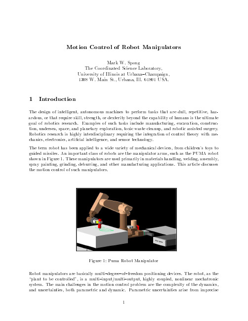
Figure 1: Puma Robot Manipulator Robot manipulators are basically multi{degree{of{freedom positioning devices. The robot, as the \plant to be controlled", is a multi{input/multi{output, highly coupled, nonlinear mechatronic system. The main challenges in the motion control problem are the complexity of the dynamics, and uncertainties, both parametric and dynamic. Parametric uncertainties arise from imprecise 1
Motion Control of Robot Manipulators
Mark W. Spong The Coordinated Science Laboratory, University of Illinois at Urbana{Champaign, 1308 W. Main St., Urbana, Ill. 61801 USA.
1.2 Kinematics
Kinematics refers to the geometric relationship between the motion of the robot in Joint Space and the motion of the end{e ector in Task Space without consideration of the forces that produce the motion. The Forward Kinematics Problem is to determine the mapping

机械力学中英文对照

face ring flux 正面通量face ring leakage flux 正面漏泄通量factor 因子fading memory 衰退记忆fading period 衰落周期failing stress 破坏应力failure 破坏failure condition 断裂条件faired curve 光滑曲线fairing 吝体fairway 航道fall 落下fall velocity 沉降速度falling ball method 落球法falling ball test 落球试验falling drop method 落滴法falling speed 下降速度falling sphere method 落球法falling sphere test 落球试验falling sphere viscometer 落球粘度计false front 假锋面family of aerofoil sections 翼型族family of oscillation characteristics 振荡特性曲线族family of waves 波族fan 风扇fan blade 风扇叶片fan brake 叶片式空气制动器fast fourier transformation 快速傅里叶变换fatigue 疲劳fatigue bending machine 弯曲疲劳试验机fatigue bending test 弯曲疲劳试验fatigue breakdown 疲劳破坏fatigue corrosion 疲劳腐蚀fatigue crack 疲劳裂缝fatigue curve 疲劳曲线fatigue damage 疲劳损伤fatigue effect 疲劳效应fatigue experiment 疲劳试验fatigue failure 疲劳破坏fatigue fracture 疲劳断口fatigue impact test 疲劳冲辉验fatigue impact testing machine 疲劳冲辉验机fatigue life 疲劳寿命fatigue limit 疲劳极限fatigue load 疲劳载荷fatigue proof 耐疲劳的fatigue resistant 耐疲劳的fatigue strength 疲劳强度fatigue test 疲劳试验fatigue testing machine 疲劳试验机fatigue wear 疲劳磨损fault 断层fault diagnosis 故障诊断fault plane 断层面faye effect 费耶效应feed 进给feed motion 进给运动feedback 反馈feedback control 反馈控制feeding power 馈给功率feeding speed 进给速度fence 挡板ferro magnetofluid dynamics 铁磁铃力学fiber composite material 纤维复合材料fibrillar structure 纤维结构fibroelastic 纤维弹性的fibrous fracture 纤维裂面fibrous structure 纤维结构fick's law of diffusion 斐克扩散定律fictitious boundary 假想边界fictitious force 表观力fictitious load 假负载fictitious pendulum 虚摆fiducial value 比较值field 场field balancing 现场平衡field decay 场衰变field density 场密度field displacement 场位移field distribution 场的分布field flutter 场的颤动field intensity 场强度field of forces 力场field of gravity 重力场field of pressure grade 压强梯度场field strength 场强度field structure 场的结构field test 现场试验field theory 场沦film boiling 膜状沸腾film effect 薄膜效应film heat transfer coefficient 膜传热系数film thickness 薄膜厚度film viscosity 薄膜粘滞性filter 过滤器filtering 过滤filtration 过滤fin 垂直稳定面final compression pressure 压缩终压力final mass 末级质量final pressure 最终压力final state 末态final strength 强度极限fine adjustment 精细蝶fine grained fracture 细晶断口fine slip 微滑移fine structure 精细结构finishing temperature 最终温度finite amplitude wave 有限振幅波finite deformation 有限形变finite difference method 有限差分法finite difference scheme 有限差分格式finite dimensional 有限维的finite dimensional space 有限维空间finite displacement 有限位移finite elasticity theory 有限弹性理论finite element 有限元finite element discretization 有限元离散化finite element method 有限元法finite element modelling 有限元模拟finite movement 有限运动finite part 有限部分finite quantity 有限量finite rotation 有限旋转finite strain 有限应变finite strip method 有限条分法firing 点火firing angle 点火角firing delay 点火延迟firing duration 燃烧持续时间firing pressure 燃烧压力firing time 点火时间first approximation 一级近似first class constraint 第一类约束first collision correction 第一次碰撞改正first cosmic velocity 第一宇宙速度first integral 初积分first law of dynamics 动力学第一定律first law of kepler 开普勒第一定律first law of thermodynamics 热力学第一定律first moment 静力矩first moment of the surface 静力表面矩first order temperature coefficient 一级温度系数first problem of dynamics 动力学第一问题first wave 一级浪fissure 裂痕fixation 固定fixed arch 固定拱fixed axoid 固定锥面fixed beam 固定梁fixed bearing 固定支承fixed bed 固定床fixed blade 固定叶片fixed center 死顶尖fixed centrode 定瞬心迹fixed coordinate system 固定坐标系fixed end 固定端fixed end arch 固定端拱fixed ended beam 固端梁fixed error 系统误差fixed frame 固定参考系fixed frequency oscillator 定频振荡器fixed in space 固定于空间的fixed in the earth coordinate system 固定于地球的坐标系fixed joint 固定连接fixed load 固定负载fixed nozzle 固定喷嘴fixed point method 不动点法fixed reference system 固定参考系fixed support 固定支点fixed vane 固定叶片fixed vector 固定矢量fixed weir 固定坝flame front 火焰头flame propagation 火焰传播flame temperature 火焰温度flange 法兰flap 襟翼flap nozzle 活动喷嘴flat jet 扁平射流flat plate 平板flat plate flow 平板绕流flat profile 平板翼型flat slab 平板flat surface 平面flattening 压扁flaw 裂纹flaw detection 探伤检验flaw detector 探伤仪flex point 拐点flexibility 挠性flexibility method 柔度法flexibility of column 柱的柔度flexibility of spring 弹簧挠性flexible 可挠的flexible coupling 挠性联轴节flexible gyroscope 挠性陀螺仪flexible plate 挠性板flexible rotor 挠性转子flexible shaft 挠性轴flexible support 挠性支承flexural buckling 屈曲flexural center 弯曲中心flexural critical speed 临界挠曲速度flexural load 弯曲载荷flexural member 受弯构件flexural modulus 弯曲模量flexural moment 弯矩flexural plane 挠曲线平面flexural rigidity 弯曲刚性flexural rigidity of the plate 板的抗弯刚度flexural strain 弯曲应变flexural strength 抗弯强度flexural stress 弯曲应力flexural vibration 弯曲振动flexural wave 弯曲波flexure 挠曲flexure of sheet 薄板挠曲flexure vibration 弯曲振动flight 飞行flight dynamics 飞行动力学flight mechanics 飞行力学flight path 飞行路径flight speed 飞行速率flight time 飞行时间flip flop oscillator 触发振荡器float 浮子float type pressure gage 浮式压力计floatability 漂浮性floatation 漂浮floatation plane 浮面floated gyroscope 液浮陀螺仪floating body 浮体floating point 浮点floating potential 浮动电位floating speed 浮动速率flocculation 凝聚flood tide 涨潮flood wave 洪水波flooding 液泛floor of ocean 海底flop in method 增加法flop out method 缩减法flow 怜flow along a slab 沿平板怜flow around 环流绕流flow around a parabola 抛物线体绕流flow around an edge 棱缘绕流flow around joukowski wing 儒科夫斯基翼绕流flow around the corner 拐角怜flow at subsonic velocity 亚声速流flow at the lifting surface 升力面上的怜flow characteristic 怜特性flow chart 撂图flow cleavage 咙理flow coefficient 量系数flow condition of hencky 亨基怜状态flow condition of mises 米泽斯屈服条件flow cone 怜锥flow curve 怜曲线flow diagram 撂图flow direction meter 怜方向仪flow ellipse 怜椭圆flow energy 怜能量flow field electrical analogy 痢电比拟flow function 量函数flow gage 量计flow height 怜指数flow in three dimensions 三维怜flow index 怜指数flow integral 怜积分flow line 吝flow machine 铃动力机flow measurement 量测定flow meter 量计flow model 怜模型flow near the wall 近壁怜flow net 柳flow nozzle 量喷嘴flow of bubble 气泡怜flow of gas 气流flow of material 物质流flow pattern 镣flow phenomenon 怜现象flow point 零flow potential 怜势flow pressure 怜压力flow profile 怜剖面图flow rate 量flow reattachment 气临附flow regime 怜状态flow regulator 量第器flow stress 怜应力flow structure 疗结构flow tube 淋flow vector 粮量flow velocity 临flow visualization 怜显示flow with heat convection 热对怜flow without separation 无分离怜flowability of solids 固体怜性flowage 蠕变fluctuating liquid drop 振荡液滴fluctuating load 变动载荷fluctuating stress 变应力fluctuation 起伏fluctuation velocity 脉动速度fluid 铃fluid clutch 液压离合器fluid dynamics 铃动力学fluid element 铃元fluid filament 细水流量fluid film 铃膜fluid flow 铃怜fluid flow efficiency 怜效率fluid flow physics 铃怜物理fluid friction 铃摩擦fluid friction damping 液体摩擦阻尼fluid kinematics 铃运动学fluid line 铃线fluid lubrication 铃润滑fluid mechanics 铃力学fluid motion 铃运动fluid phase 液相fluid plastic 猎塑料fluid pressure 铃压力fluid surface 伶fluid type instability 铃型不稳定性fluid wave 铃波fluidal 铃的fluidal structure 疗结构fluidic 铃的fluidic element 铃元fluidity 怜性fluidity coefficient 寥fluidization 连化fluidized bed 怜床flume 水沟道flute type deformation 槽型形变flutter 颤振flutter of aerofoil 机翼颤振flux 通量flux density 通量密度flux equilibrium 通量平衡flux of force 力线通量flux peak 最大通量flying height 飞行高度flying range 航程flying speed 飞行速度flywheel 惯性轮flywheel effect 飞轮效应flywheel fan 飞轮风扇flywheel moment 飞轮力矩foam 泡沫foaming 发泡focal length 焦距focal length ratio 焦距比focal plane 焦面focus of earthquake 震源fokker planck collision term 福克尔普朗克碰撞项fokker planck equation 福克尔普朗克方程folded plate structure 折板结构folded system 折板结构folding 弯曲folding strength 曲折强度folding test 曲折试验follow rest 移动中心架following 追踪following wake 伴流foot 底座force 力force analysis 受力分析force coefficient 力系数force constant 力常数force couple 力偶force density 力密度force dependent on position 与位置依赖的力force dependent on velocity 与速度依赖的力force diagram 力图force distribution 力分布force feed 压力进给force field 力场force free 未受力酌的force function 力函数force in member 构件力force in the bar 杆内酌力force of attraction 引力force of gravity 重力force of inertia 惯性力force of repulsion 斥力force operator 力算符force pipe 压力管force polygon 力多边形force polygon rule 力多边形法force pump 压力泵force sensing of robot 机扑的力感度force sensor 力传感器force system 力系force system of equal effect 等效力系force triangle 力三角形force unbalance 力不平衡force vector 力矢量force voltage analogy 力电压模拟forced circulation 强制循环forced convection 强制对流forced convection air cooler 强制对琳气冷却器forced diffusion 强制扩散forced draught 强制通风forced emission 受迫发射forced oscillations 受迫振荡forced regular precession 强迫规则旋进forced ventilation 强迫通风forced vibration 受迫振荡forced vortex 强制旋涡forced wave 强制波forcing screw 加压螺钉foreshock 前震form drag 形阻力form of bifurcation 分叉形状form of energy 能量形式form of oscillations 振荡形式form of vibrations 振荡形式form resistance 形阻力formation energy 形成能formation enthalpy 形成焓formation entropy 形成熵formation heat 形成热formation of eddy 涡旋形成formation of thermal cracks 热裂形成formation of vortices 涡旋形成formation of waves 波的形成forming 成形forward difference 前向差分forward direction 正向forward movement 前向运动forward scattering 前方散射forward scattering angle 前方散射角forward scattering peak 前方散射峰forward speed 前进速度forward velocity 前进速度forward wave 前向波foucault gyrocompass 傅科陀螺仪foucault pendulum 傅科摆foucault pendulum experiment 傅科摆实验foundation slab 基础底板fountain effect 喷注效应four dimensional force 四维力four dimensional velocity 四维速度four dimensional wave vector 四维波矢量fourier component 傅里叶分量fourier expansion 傅里叶展开fourier integral 傅里叶积分fourier law 傅里叶定律fourier series 傅里叶级数fourier transform 傅里叶变换fourier transformation 傅里叶变换fractional fissure 断裂纹fractural cleavage 破劈理fracture 断裂fracture appearance 断口外观fracture condition 断裂条件fracture criterion 断裂准则fracture dynamics 断裂动力学fracture face 破坏面fracture load 断裂载荷fracture mechanics 断裂力学fracture strain 断裂应变fracture surface 破坏面fracture test 断裂试验fracture toughness 断裂韧性fracturing load 断裂载荷fragility 易碎性fragment 碎片fragmentation 破碎frame 框架frame of reference 参考系frame structure 框架结构framework 框架framework method 框架法framing index 照准标志free air effect 自由空气效应free air overpressure 自由大气超压free boundary 自由边界free boundary flow 自由边界流free convection 自由对流free edge 自由边free end 自由端free energy 自由能free energy density 自由能密度free energy function 自由能函数free enthalpy 自由焓free fall 自由下降free fall apparatus 自由降落装置free fall trajectory 自由降落轨道free fall weir 自两溢吝free falling body 自由落体free flight 自由飞行free flow 自由怜free head 自由水头free internal rotation 自由内转动free jet 自由射流free jet wind tunnel 自由喷射风洞free length 自由长度free mass point 自由质点free meander 自由曲流free molecule flow 自由分子流free motion 自由运动free oscillation 自由振荡free outflow 自由瘤free path 自由程free pendulum 自由摆free period 自由周期free plastic flow 自由塑性怜free regular precession 自由规则旋进free rotation 自由旋转free rotor 自由转子free rotor gyroscope 自由转子陀螺仪free running oscillator 自激振荡器free space 自由空间free space propagation 自由空间传播free spinning 旋转free spinning tunnel 旋转竖直风洞free stream 自由怜free stream mach number 自由另赫数free stream velocity 自由怜速度free surface flow 自由表面怜free surface of water 自由水面free surface vortex 自由面涡free surface wave 自由表面波free time of flight 自由飞行时间free torsion 自由扭转free vector 自由矢量free vibration 自由振荡free volume 自由体积free volume theory 自由体积理论free vortex 自由涡free vortex system 自由涡恋free wave 自由波freedom of motion 运动的自由度freely supported 自由支承的freezing 凝固freezing method 冻结方法freezing point 凝固点freezing temperature 冻结温度freighter 运输机frequency 频率frequency analysis 频率分析frequency analyzer 频率分析器frequency characteristic 频率特性frequency conversion 频率转换frequency distribution 频率分布frequency division 分频frequency domain 频率范围frequency domain method 频域法frequency drift 频率偏移frequency factor 频率因数frequency instability 频率不稳定性frequency jumping 频率跃变frequency meter 频率计frequency method 频率法frequency modulation 频率灯frequency of fadings 衰减频率frequency of ripple 脉动频率frequency parameter 频率参数frequency range 频率范围frequency response 频率响应frequency spectrum 频谱frequency stability 频率稳定度frequency standard 频率标准frequency synthesis 频率合成fresh water 淡水fresh wind 清风friability 易碎性friction 摩擦friction angle 摩擦角friction brake 摩擦闸friction circle 摩擦圆friction coefficient 摩擦系数friction cone 摩擦圆锥friction constant 摩擦常数friction damper 摩擦减震器friction depth 摩擦深度friction drag 摩擦阻力friction drum 摩擦滚筒friction factor 摩擦系数friction gage 摩擦压力计friction head 摩擦水头friction layer 摩擦层friction moment 摩擦力矩friction of motion 运动摩擦friction of rest 静摩擦friction pendulum 摩擦摆friction resistance 摩擦阻力friction roller 摩擦轮friction shock absorber 摩擦式减振器friction spring 摩擦弹簧friction stress 摩擦应力friction surface 摩擦面friction tensor 摩擦应力张量friction term 摩擦项friction velocity 摩擦速度frictional compensation 摩擦补偿frictional error 摩擦误差frictional force 摩擦力frictional heat 摩擦热frictional loss 摩擦损耗frictional oscillation 摩擦振荡frictional ratio 摩擦比frictional resistance 摩擦阻力frictional work 摩擦功frictionless 无摩擦的frictionless instability 非粘性粱稳定性friedrich diagram 弗里德利希示意图fringe density 条纹密度front 锋面front of the detonation wave 爆震波波前front wave 锋面波front wing 前翼frontal drag 迎面阻力frontal edge 前缘frontal resistance 迎面阻力froude pendulum 弗劳德摆frozen equilibrium 冻结平衡frozen flow 冻结怜frozen in degree of freedom 冻结自由度frozen in field lines 冻结力线frozen in magnetic field 冻结磁场frozen soil 冻土fuel 燃料fulcrum 支点fulcrum of suspension 悬挂点full flow 总量full load 全负荷full power 全功率full scale 实际缩尺full sphere 实心球full wave 全波fully developed turbulence 完全发达湍流fully elastic 完全弹性的fully elastic torsion 完全弹性扭转fully ionized plasma 完全电离等离子体fully plastic 完全塑性的fully plastic torsion 完全塑性扭转fume 烟雾function of bounded variation 有界变分函数function of strain 应变函数functional determinant 函数行列式functional equation 函数方程functional model 函数模型functional similarity 函数相似functional simulation 函数模拟fundamental equation 基本方程fundamental frequency 基频fundamental harmonic 基谐波fundamental matrix 基本矩阵fundamental oscillation 基本振动fundamental resonance 基频谐振fundamental tensor 基本张量fundamental vibration 基本振动fundamental wave 基波fundamental wavelength 基波长funicular polygon 肃边形funnel viscometer 漏斗形粘度计fuzzy optimization 模糊优化fuzzy random vibration 模糊随机振动。

操作工程机器人改进力反馈控制方法

吉椿大学学报（工学版）
第３８卷
利用图７所示的实验平台，分别在空载、弹
簧、刚洼受载情况下，霹本文静改进塑力反馈双囊
（１３）
伺服控制方法的有效性进行验证。空载时，主要
３．３．３增量式ＰＩＤ系数的调整方法系统误差
观察从手对主手位移的跟踪性能，熟次通过观察主手操缀力豹变纯情嚣，霹泼检验ＲＢＦ—ＰＩＤ蘩力
３反馈增益系数和主手力控制器
３．１反馈增益系数设计
蓠先，在鼠耱羟一化餐值ｌ疋｜论域上定义３个模糊子集：ＢＩＧ，ＭＩＤ，ＳＭＬ；模糊子集的隶属度函数选择为垒交叠连续线性梯形，如图４所示。模寮映射麓赠为：
Ｒ１：ＩＦＥｆｉｓＢＩＧＴｈｅｎＫｅｎ一０．５Ｒ２：ＩＦＦｅＩｉｓＭＩＤＴｈｅｎＫｅｆ２一ｌ必３：ｌＦ｜疋｜ｉｓＳＭＬＴｈｅｎ鬈ｅｆ３—２采用代数积一重心法推理规则，得Ｔ—Ｓ型模糊反馈增益Ｋｅｆ的非线性化救线如图５所示。
Ｘ＝［ｚｌ，ｚ２，ｚ３，ｚ４，ｚ５，ｚ６］Ｔ
式中：ｚ。＝Ａｕ（忌）为ｋ时刻实际系统控制量的变
化量ｆｚ２一“（是一１）；ｚ３一“（忌一２）；ｚ４＝Ｙ（忌）；ｚ５
一ｙ（矗一１）；３２。一ｙ（忌一２）分别表示系统在相应时
刻的输出值和控制量。
ｈｉ—ｐ（一掣）萨ｍ，…，８隐层节点取高斯核函数
式中：第＿ｆ个节点ｈ，的中心向量ｃ，一［ｏ。，ｆ，ｚ， …，ｃ，。］Ｔ；基宽度６＝［６。，ｂ：，…，ｂ。］Ｔ；节点向量Ｈ一［＾１，ｈ２，…，矗８］Ｔ。
既能保证从手对盘手的位置跟随精度，叉能使主簪连续的跟随从手受力情况，减小了反馈力冲
击现象，增加了力反馈的平顺性。提高了力反馈遥操作工程机器入系统的操作性能和透明度。
关键词；流体传动专控镧；模灏交增益茂馕系数；力反馈；遥攮作王程机器人

Haptic Feedback Robot Control

Haptic Feedback Robot ControlHaptic feedback is a crucial aspect of robot control, as it allows for the transmission of information through touch, enabling the operator to interact with the robot and perceive its environment. However, there are several challenges associated with haptic feedback robot control that need to be addressed in order to improve its effectiveness and usability.One of the main challenges is the design of haptic feedback systems that can accurately convey information to the operator. This requires the development of advanced sensors and actuators that can detect and transmit tactile information in real-time. Additionally, the haptic interface needs to be carefully designed to ensure that the operator can interpret the feedback intuitively and effectively.Another challenge is the integration of haptic feedback with other forms of feedback, such as visual and auditory cues. This requires careful coordination and synchronization of different sensory inputs to provide a coherent and comprehensive perception of the robot's actions and surroundings. Furthermore, the haptic feedback needs to be prioritized and presented in a way that complements the other feedback modalities, rather than overwhelming or conflicting with them.In addition to technical challenges, there are also ergonomic and usability considerations that need to be taken into account. The haptic interface should be designed to be comfortable and intuitive to use, allowing the operator to control the robot with precision and ease. This involves considerations such as the size and shape of the haptic device, the placement of tactile sensors and actuators, and the overall ergonomics of the control interface.Furthermore, there are safety considerations associated with haptic feedback robot control. The haptic interface needs to be designed in a way that minimizes the risk of accidental injury or damage, both to the operator and the robot itself. This requires the implementation of safety features and fail-safes, as well as thorough testing and validation of the haptic control system.Another important aspect to consider is the psychological and cognitive factors involved in haptic feedback robot control. The haptic interface should be designed to provide a natural and intuitive interaction experience, minimizing cognitive load and mental fatigue for the operator. This involves considerations such as the mapping of tactile feedback to the operator's mental model of the robot and its environment, as well as the provision of clear and meaningful haptic cues.Lastly, there are broader societal and ethical considerations associated with haptic feedback robot control. As robots become increasingly integrated into various aspects of our lives, it is important to consider the impact of haptic feedback on human-robot interaction and the potential implications for social and ethical norms. This involves considerations such as the design of haptic interfaces that promote trust and collaboration between humans and robots, as well as the establishment of guidelines and regulations for the use of haptic feedback in robotic systems.In conclusion, haptic feedback robot control presents a range of technical, ergonomic, safety, psychological, and societal challenges that need to be carefully considered and addressed in order to realize its full potential. By taking a holistic and interdisciplinary approach to the design and implementation of haptic feedback systems, we can create more intuitive, effective, and ethical human-robot interaction experiences.。

第10章力控与顺应控制

• 位置/力混和控制（ Hybrid Position/Force Control ）位置力混和控制（力混和控制
位置/力混和控制是由Raibert and Craig 在1981年提出的它的思想是分别将机器人的力控和位置控制在控制器的两个不同通道上实现，这就是著名的 R－C控制器。其代表作是： • M H Raibert and J J Craig. Hybrid Position/Force control of Manipulators. Trans, of ASME, Journal of DSMC, Vol. 102, June 1981. pp.126-133
2011年 2011年3月13日 13日
天津工程师范学院机械工程系
7
真正将力控用于多关节机器人上的是Whitney，他在1977年将力传感器用在多关节机器人上，并用解运动速度的方法（RMRC）推导出力反馈控制的向量表达式。而R.P.Paul（1972）和Silver（1973）则分别用选择自由关节（free joints）的方法实现对机器人力的开环控制。见下文： • 见RMPC列举的文（1） • D Silver. The little Robot System. AIM-73, Cambridge, MIT, Artificial Intelligence Lab., 1973 1976年R. P. Paul 和 B. Shimano进一步完善上述方法，采用腕力传感器实现对机器人力的闭环控制。见下文： • R P Paul and B Shimano. Compliance and Control. Proc. Joint Automatic control, Conf. Sam Francisco, IEEE, pp694-699, 1976

三维环境下基于反步法的多机器人编队控制

三维环境下基于反步法的多机器人编队控制冯磊;肖伸平【摘要】针对两轮式移动机器人在复杂环境下的编队控制问题,提出一种基于虚构领航法和反步法,并结合人工势场法策略的多机器人避障编队算法.首先,详细分析多机器人系统在三维空间下的编队模型,并利用空间投影方法将其映射到二维平面进行分析.其次,将运动学模型转化为链式形式,并通过正则坐标变换,将误差系统形式转换成串联非线性系统.然后运用Backstepping方法构造轮式机器人追踪系统的Lyapunov函数,设计出针对轮式机器人的轨迹跟踪控制器.再结合人工势场法避障策略,完成多机器人复杂环境下的编队任务.最后,通过多机器人轨迹跟踪的两组仿真实验,验证了所提出方法的有效性.【期刊名称】《湖南工业大学学报》【年(卷),期】2017(031)001【总页数】6页(P69-74)【关键词】三维空间;人工势场法;反步法;李雅普诺夫函数;编队控制【作者】冯磊;肖伸平【作者单位】湖南工业大学电气与信息工程学院,湖南株洲 412007;湖南工业大学电气与信息工程学院,湖南株洲 412007【正文语种】中文【中图分类】TP273近年来，随着机器人技术的发展，多机器人的稳定控制和轨迹跟踪问题越来越受到国内外学者的关注[1]。

相对于稳定问题，轨迹跟踪是一个更实际的控制问题。

而编队往往将面对复杂的环境，因此，在障碍物环境下，迫切需要寻找一条从起始位置到达目标位置的避障路径。

而路径规划中的人工势场法以其数学计算简单明了而被广泛应用。

目前，国内外学者进行编队研究的机器人主要有地面自主移动机器人、水下自主式机器人、卫星和无人飞行器等[2-3]；多机器人的控制算法主要包括虚拟结构法、领航跟随法、图论法和基于行为的方法[4-6]。

在当前的研究中，文献[7]综合路径跟踪法和虚拟结构法，实现了多机器人系统的动态编队控制。

其缺点是其虚拟结构运动的队形要求限制了该方法的应用范围，难以实现灵活的队形控制。

基于外环速度补偿的封闭机器人确定学习控制

基于外环速度补偿的封闭机器人确定学习控制王敏 1, 2林梓欣 1王聪 3杨辰光1摘要针对未开放力矩控制接口的一类封闭机器人系统, 提出一种基于外环速度补偿的确定学习控制方案. 该控制方案考虑机器人受到未知动力学影响, 且具有未知内环比例积分(Proportional-integral, PI)速度控制器. 首先, 利用宽度径向基函数(Radial basis function, RBF)神经网络对封闭机器人的内部未知动态进行逼近, 设计外环自适应神经网络速度控制指令. 在实现封闭机器人稳定控制的基础上, 结合确定学习理论证明了宽度RBF 神经网络的学习能力, 提出基于确定学习的高精度速度控制指令. 该控制方案能够保证被控封闭机器人系统的所有信号最终一致有界且跟踪误差收敛于零的小邻域内. 在所提控制方案中, 通过引入外环补偿控制思想和宽度神经网络动态增量节点方式, 减小了设备计算负荷, 提高了速度控制下机器人的运动性能, 解决了市场上封闭机器人系统难以设计力矩控制的难题, 实现了不同工作任务下的高精度控制. 最后数值系统仿真结果和UR5机器人实验结果验证了该方案的有效性.关键词确定学习, 速度补偿控制, 神经网络, 封闭机器人引用格式王敏, 林梓欣, 王聪, 杨辰光. 基于外环速度补偿的封闭机器人确定学习控制. 自动化学报, 2023, 49(9): 1904−1914DOI 10.16383/j.aas.c220575Deterministic Learning of Manipulators With Closed ArchitectureBased on Outer-loop Speed Compensation ControlWANG Min 1, 2 LIN Zi-Xin 1 WANG Cong 3 YANG Chen-Guang 1Abstract In this paper, a deterministic learning outer-loop speed compensation control scheme is proposed for a class of manipulator systems with closed architecture and without open torque control interface. The proposed scheme focuses on that the manipulator is affected by unknown modelling dynamics and has an unknown inner-loop proportional-integral (PI) speed controller. Firstly, the broad radial basis function (RBF) neural network is used to approximate the internal unknown dynamics of the manipulator with closed architecture, and the outer-loop adapt-ive neural network speed control command is designed by using the Lyapunov function. Based on the stable control of man-ipulator with closed architecture, the dynamic learning ability of RBF neural network is verified, and then the high-accuracy speed control command is designed based on the deterministic learning theory. The proposed control sch-eme guarantees that all signals of the manipulator system with closed architecture are ultimately uniformly boun-ded, and the tracking error converges to a small neighborhood of zero. By the combination of outer-loop compensa-tion control and dynamic incremental node of broad neural networks, the proposed scheme reduces the computing lo-ad, improves the motion performance of the robot under speed control, solves the torque control design difficulty of the closed manipulator, and realizes high-precision control in different working tasks. Finally, simulation results of numerical system and experimental results of UR5 robot are used to show the effectiveness of the proposed scheme.Key words Deterministic learning, speed compensation control, neural network, manipulators with closed architec-tureCitation Wang Min, Lin Zi-Xin, Wang Cong, Yang Chen-Guang. Deterministic learning of manipulators with closed architecture based on outer-loop speed compensation control. Acta Automatica Sinica , 2023, 49(9):1904−1914近年来, 机器人在工程应用和日常生活中发挥着越来越重要的作用, 被广泛应用于空间探测、焊收稿日期 2022-07-14 录用日期 2023-01-11Manuscript received July 14, 2022; accepted January 11, 2023国家自然科学基金(62273156, 61890922, U20A20200, 61973129), 广东省自然科学基金(2019B151502058), 鹏城实验室重大攻关项目(PCL2021A09), 佛山市科技攻关项目(2020001006308,2020001006496)资助Supported by National Natural Science Foundation of China (62273156, 61890922, U20A20200, 61973129), Natural Science Foundation of Guangdong Province (2019B151502058), the Ma-jor Key Project of Peng Cheng Laboratory (PCL2021A09), and Industrial Key Technologies Program of Foshan (2020001006308,2020001006496)本文责任编委许斌Recommended by Associate Editor XU Bin1. 华南理工大学自动化科学与工程学院广州 5106412. 鹏城实验室深圳 5180553. 山东大学控制科学与工程学院济南2500611. School of Automation Science and Engineering, South China University of Technology, Guangzhou 5106412. Peng Cheng Laboratory, Shenzhen 5180553. School of Control Science and Engineering, Shandong University, Jinan 250061第 49 卷第 9 期自动化学报Vol. 49, No. 92023 年 9 月ACTA AUTOMATICA SINICASeptember, 2023接、装配、医疗等领域, 相关技术也越来越受到科研人员重视[1−3]. 在机器人控制领域, 其控制目标之一就是实现机器人对特定任务轨迹的跟踪. 多自由度机器人作为一个高度耦合的非线性多输入多输出系统[4], 主要控制难点在于机器人工作环境任务多变,在外界扰动、负载变化、参数测量不精确等因素影响下, 机器人系统精确建模难度较大, 使得比例积分微分(Proportional-integral-derivative, PID)控制等经典控制算法难以满足机器人控制的精度要求. 针对机器人系统存在部分参数不确定或测量不准确的问题, 一些学者结合鲁棒控制、滑模控制等思想, 提出了许多有效的自适应控制算法[5−7]. 当机器人系统存在不可建模动态时, 一些学者结合神经网络的非线性函数逼近特性, 提出了大量的自适应神经网络控制方案, 保证了机器人在多变环境下的高性能控制[8−12].值得注意的是, 上述控制方案大多数都是基于力矩进行控制器设计, 其方案有效性主要是通过数值系统仿真进行验证, 鲜有在实际机器人上进行实验和应用. 造成上述现象的原因是, 当前市面上大部分工业/商业机器人并不开放力矩接口, 而是采用速度/位置控制. 这些封闭机器人采用标准的内外环控制结构, 其中外环为运动学环, 内环为动力学环, 内环控制的采样速率一般比外环要快得多,且普遍认为其内环控制使用速度比例积分(Propor-tional-integral, PI)控制器或位置PID控制器[13].封闭机器人的这些性质, 导致用户一般只能对其进行简单的运动学控制[14], 从而使得机器人难以应对多变的个性化产品加工. 针对这类具有内外环结构的机器人的控制问题, 部分学者提出了解决方案.文献[5, 15]在研究具有未知动力学和未知运动学的机械臂控制时, 提出了适当的自适应控制器. 文献[16]研究了一类具有关节速度反馈内环的机器人任务空间控制问题, 提出了一种基于模型的内环关节速度控制器通用结构[17]. 注意到, 上述控制方案中跟踪误差的收敛依赖于内环速度控制器的修改或再设计, 并不是常见的速度PI控制器或位置PID控制器, 对于具有不可修改内环的工业/商业机器人而言, 这些控制方案也难以实现应用. 进一步, 一些学者提出了预校正方案[18], 这些预校正方案的有效性验证主要是通过直观解释和实验结果进行的, 并没有进行严格理论分析. 针对封闭机器人控制存在的上述问题, 文献[19]在考虑机器人具有可以线性参数化的未知动力学和运动学且内环控制器参数未知和不可修改的背景下, 设计了一类外环自适应速度补偿控制器, 保证了机器人系统的稳定性和误差收敛. 该方案需要计算动力学和运动学回归矩阵, 这两个矩阵随着机械臂关节增多, 计算的复杂度呈指数倍增长. 此外, 实际机器人系统由于受到阻尼以及摩擦力等影响, 存在本质的非线性. 因此, 如何提出简单有效的封闭机器人控制方案, 既能实现封闭力矩的补偿控制, 又能精确建模未知非线性仍是一个开放性的问题.众所周知, 神经网络是建模未知非线性的有效方法[20]. 然而, 现有的大部分自适应神经网络控制并没有充分利用神经网络的学习能力, 即使是处理相同的任务也需要对神经网络进行重复训练, 该过程耗时长、计算资源消耗大、暂态阶段的控制性能也较差. 因此, 如何实现神经网络在控制过程中的学习和经验知识再利用是一个很有意义的课题[21].对此, 文献[22]提出确定学习理论, 解决了神经网络对未知动态的学习问题. 该理论证明了沿着回归轨迹的径向基函数(Radial basis function, RBF)神经网络满足持续激励(Persistent excitation, PE)条件, 进一步结合线性时变系统指数稳定性证明了神经网络权值的精确收敛. 基于该理论, 文献[23]引入动态面技术, 解决了自适应神经网络在严格反馈系统中的学习问题. 近年来, 确定学习理论也已被广泛应用于机器人编队控制[24]、心肌缺血早期诊断[25]、水面无人船控制[26]等领域, 在机械臂控制领域也有相关工作[27]. 然而, 现有基于确定学习的控制方案仍是基于力矩进行设计的, 无法在封闭的工业/商业机器人上直接进行应用.综上所述, 本文针对未开放力矩接口的一类封闭机器人系统, 在考虑机器人受到未知动力学影响且具有未知内环PI速度控制器的情况下, 基于文献[19]的外环补偿框架提出了一种基于外环速度补偿的确定学习控制方案, 实现了封闭机器人的关节轨迹跟踪控制. 该方案的主要贡献点如下: 1)在文献[19]的工作基础上, 引入神经网络处理系统未知动态, 取消了封闭机器人未知动力学模型参数线性化假设, 并简化了外环补偿控制设计过程; 2)采用宽度RBF神经网络动态增量神经网络节点, 降低了网络结构复杂度, 改善了系统控制的实时性;3)引入确定学习理论, 实现了宽度RBF神经网络对封闭机器人未知动态的精确学习, 并利用经验知识避免了对网络重复训练, 降低了计算负担, 实现了快稳准的高精度跟踪控制; 4)为确定学习理论应用于具有类似结构的封闭机械系统提供了研究思路, 拓展了确定学习的应用范围.1 问题描述及预备知识1.1 系统说明与控制目标n 本文所考虑的由永磁直流电动机驱动的自由9 期王敏等: 基于外环速度补偿的封闭机器人确定学习控制1905度机器人动力学模型[19]如下x 1∈R n M (x 1)∈R n ×nC (x 1,˙x1)∈R n ×n G (x 1)∈R n K ∈R n ×n u ∈R n 其中, 是机器人关节角位置; 是机器人的惯性矩阵; 是机器人的科氏力矩阵; 是机器人的重力向量; 是机器人内部的控制增益, 为一常值对角正定矩阵; 是封闭机器人的内环控制器.M (x 1)λm λM λm I ≤M (x 1)≤λM I I 性质 1. 机器人动力学方程的惯性矩阵是对称并一致正定的, 且具有一致的界限, 存在正常数和使得 , 其中为适当定义的单位矩阵.C (x 1,˙x 1)˙M (x 1)−2C (x 1,˙x 1)性质 2. 可以通过适当定义机器人动力学方程的科氏力矩阵 , 使得是斜对称矩阵.在研究的封闭机器人内外环控制方法中, 本文考虑内环控制器为PI 速度控制器[19], 结构如下˙q c q c K p K i 其中, 和是关节速度指令和关节位置指令, 是内环控制器的比例系数, 是内环控制器的积分系数, 均为未知对角正定矩阵.考虑如下光滑有界参考模型, 该模型将产生封闭机器人的关节期望轨迹x d 1∈R n x d 2∈R n f (x d 1,x d 2)y d =x d 1y d 其中, 和分别是封闭机器人期望的关节角位置和角速度, 是给定的光滑非线性函数, 是封闭机器人期望输出. 本文假设期望输出为周期轨迹.本文的控制目标是基于外环速度补偿控制思想, 在考虑封闭机器人具有不确定动力学和未知参数内环控制器的情况下设计系统(1)的速度控制指x 1y d 令, 从而确保: 1)机器人系统的所有信号都是最终一致有界的; 2)系统的输出能够跟踪给定的期望输出轨迹 ; 3)在控制过程中学习机器人内部未知动态, 并利用学到的未知动态知识实现封闭机器人高精度跟踪控制. 控制方案框图如图1所示.1.2 RBF 神经网络1) RBF 神经网络的万能逼近特性: 为逼近机械臂控制过程中的未知非线性动态, 本文使用如下形式的RBF 神经网络f (Z )∈R n Z ∈ΩZ ΩZ W ∗∈R np p S (Z )=[s 1(Z −ξ1),···,s p (Z −ξp )]T s i (Z −ξi )=exp (−(Z −ξi )T (Z −ξi )/ηi )ξi =[ξi 1,···,ξin ]T ηi ϵ(Z )ΩZ f (Z )∥ϵ(Z )∥≤ϵ∗ϵ∗其中, , 是神经网络输入向量, 为一紧集, 是神经网络理想权值向量, 为RBF 神经网络隐含层节点数, 为回归向量, 此处选取高斯函数作为径向基函数, 和分别是神经元节点的中心和宽度, 是RBF 神经网络逼近误差. 文献[28]已经证明通过选取适当的神经元节点数、神经元中心和宽度, RBF 神经网络能够以任意精度逼近在紧集上的任意光滑连续函数 , 即逼近误差 , 是一个任意小的正整数.ΩZ Z f (Z )2) RBF 神经网络的局部逼近能力: 基于文献[22], 对于紧集内的任意有界轨迹 , 可以用沿着该轨迹的局部区域内有限数量的神经元逼近, 即S ζ(Z )=[s 1ζ(Z −ξ1ζ),···,s p ζ(Z −ξp ζ)]T S (Z )W ∗ζ∈R np ζW ∗p ζ<p ϵζ(Z )∥ϵζ(Z )∥−∥ϵ(Z )∥其中, 是回归向量的子向量, 是神经网络理想权值向量的子向量, 且 , 是局部RBF 神经网络逼近误差, 且是一图 1 封闭机器人控制系统框图Fig. 1 Schematic diagram of manipulators with closed architecture control system1906自动化学报49 卷个极小值.S :[0,∞)→R s Λ1,Λ2,T 0定义 1[22]. 考虑一致有界且分段连续的向量函数 , 若存在大于零的常数 ,使得如下公式成立S I s ×s那么向量函数满足PE 条件, 其中定义为维的单位矩阵.Z Z [0,∞)R q Z ΩZ ⊂R q ΩZ Z S ζ(Z )引理 1[22]. RBF 神经网络的局部PE 条件: 考虑任意回归/周期轨迹 , 假设是从到的连续映射, 且位于紧集中. 则对于中心置于规则晶格(足够大到覆盖紧集 )上的RBF 神经网络, 只有中心位于回归/周期轨迹的小邻域内的神经元才会被激励, 由其组成的回归子向量将满足PE 条件.1.3 宽度RBF 神经网络在传统的RBF 神经网络逼近中, 需通过选取合适的神经元节点数、中心和宽度来保证逼近精度,而在实际应用中通常需要设计者根据自己的经验不断试错, 采用均匀布点的方式来设计RBF 神经网络的结构, 具有很强的主观性. 同时, 机器人控制系统是一个多输入多输出系统, 随着控制连杆数量的增加, RBF 神经网络的输入维数会呈几何倍数增长, 在均匀布点的设计方案下, 神经元数量也会急剧升高, 这将导致神经网络的计算负荷提高, 对硬件设备提出了更高的要求, 同时也将影响系统控制的实时性. 为了解决上述问题, 本文将使用文献[29]所提出的宽度RBF 神经网络方法进行网络结构设计. 该方法结合宽度神经网络增量节点的思想, 可实现在系统控制过程中神经元的自适应调整.宽度RBF 神经网络在初始化阶段以系统的初始状态为第一个神经元, 之后会根据神经网络的实际输入与网络已有神经元中心的距离来判断是否应该新增神经元. 新增神经元的增加策略如下:1)定义新增神经元所需参数ξn ,ηn ,W n 其中, 分别是新增神经元的中心、宽度和权值, 本文新增神经元的宽度设置与已有神经元一致, 权值统一初始化为零.2)判断当前网络输入是否超出现有神经元所构成的紧集域k C min ={c 1,···,ck }首先, 本文使用欧氏距离来描述当前网络输入与神经元中心点的距离, 根据距离选取离当前输入最近的个点集 , 则可由下式获得新增神经元的中心βC min 0∼1¯Cmin C min ¯Cmin =(c 1+c 2+···+c k )/k 其中, 是决定新增神经元与神经元集合之间距离的可调参数, 取值范围为 ; 是神经元集合的平均中心位置, .εZ C min ¯Cmin ε然后, 设置判断是否新增神经元的可调阈值 ,当神经网络当前输入与神经元集合的平均中心位置之间距离大于阈值时, 添加新的神经元, 否则保持原有神经元集合不变.2 外环自适应神经网络速度控制指令设计本节将针对系统(1), 采用反步法进行基于外环补偿的速度控制指令设计. 首先将封闭机器人系统的内环速度PI 控制器(2)代入系统(1), 将系统(1)转化为如下形式K P =KK p K I =KK i y y =x 1其中, , , 是机器人系统输出关节角位置, .根据传统反步法设计思想, 定义如下误差变量α1α1˙q c 其中, 是虚拟控制器. 考虑系统(8), 接下来的反步设计包括两个步骤, 将依次设计出虚拟控制器和速度控制指令 . 具体设计过程如下:z 1步骤 1. 考虑系统(8)以及误差定义(9), 对求导得α1根据式(10), 虚拟控制器可设计为c 1其中, 为控制增益, 且为正的设计参数.z 2步骤 2. 根据误差定义(9), 对求导可得考虑封闭机器人系统具有未知的动力学和内环速度PI 控制器, 定义未知系统动态为Z 1=[x T 1,x T 2,q T c ,˙αT 1]T ∈R 4n n f (Z 1)其中, , 是机器人自由度. 使用RBF 神经网络来逼近未知动态 , 得9 期王敏等: 基于外环速度补偿的封闭机器人确定学习控制1907ϵ1(Z 1)∥ϵ1(Z 1)∥≤ϵ∗ϵ∗W ∗1∈R nϖϖW ∗1ˆW 1˜W 1=ˆW 1−W ∗1其中, 是逼近误差, 且 , 是任意小的正数, 是未知的理想权值向量, 为宽度RBF 神经网络节点个数. 令的估计值为, 则权值估计误差为 .将式(14)代入式(12)可得ˆW1W ∗根据式(15), 利用权值估计值代替理想权值 , 设计自适应神经网络速度控制指令如下并构造神经网络权值估计值更新率为c 2˙q c γσσ其中, 是速度控制指令的控制增益, 且为正的可设计参数; , 分别是神经网络权值估计值更新率的控制增益和修正项, 均为正的待设计参数.q c ˙qc q c 注 1. 在考虑未知动力学影响的机器人自适应神经网络控制器设计中, 现有大部分成果均为力矩控制器, 无法应用于本文所考虑的封闭机器人系统.本文在机器人具有未知不可修改内环速度PI 控制器的背景下, 设计了与内环相匹配的外环自适应神经网络速度控制指令. 该指令与常见力矩控制器的代数方程形式不同, 是一个关于的一阶微分方程,通过求解该微分方程, 可以获得输入机器人系统的速度控制指令和位置控制指令 , 同时, RBF 神经网络的应用使该速度控制指令具有适应机器人未知动力学影响和未知内环控制器的能力.q c K,K p ,K i K −1P K I q c 注 2. 与现有基于反步法的自适应神经网络力矩控制器相比, 本文所设计速度控制指令在神经网络输入上将多出一个信号 . 这是因为在控制器设计过程中, 为了处理内环速度PI 控制器的未知参数带来的不确定性, 本文在定义未知系统动态的时候将考虑在内, 从而有助于后续的控制器设计以及未知动态的精确神经网络逼近.至此, 可得封闭机器人的闭环系统动态如下µ>0V (0)≤µc 1c 2γσz 1z 2定理 1. 考虑由封闭机器人系统(8)、参考模型(3)、自适应神经网络速度控制指令(16)和神经网络权值估计值更新率(17)所组成的闭环系统, 那么对于任意给定的常数以及所有满足的系统初始状态,则通过选取合适的设计参数 ,, 和 , 可以使得闭环系统中的所有信号是最终一致有界的, 并且跟踪误差 , 能够收敛到零的小邻域内.证明. 选取如下Lyapunov 函数结合机器人动力学方程性质2, 沿系统(18)所产生的轨迹对所选Lyapunov 函数求导可得利用Young 不等式对Lyapunov 函数的导数放缩得λmin (K P )K P 其中, 是矩阵的最小特征值.结合式(19)和式(21)可得其中a >b /µV =µ˙V≤0V ≤µV (0)≤µt >0V (t )≤µ至此, 只要选择 , 那么可以保证当时, , 因此是一个不变集, 即对于任意满足的初始条件, 对于任意 , 有 .进一步, 对式(22)积分可得其中c 1,c 2,从上式可知, 通过选取合适的设计参数 1908自动化学报49 卷γ,σθ, 可使得任意小. 因此, 闭环系统中的所有信号是最终一致有界的.进一步, 从式(19)及式(23)可得ν1>√2θ/λmin (K P )ν2>√2θ/λm T 1t>T 1令 , , 则存在一个有限时间 , 对于任意有θν1,ν2z 1,z 2T 1从上述分析可知, 选取合适的设计参数可使任意小, 即可以任意小, 因此跟踪误差可以在有限时间内收敛到零的小邻域内.□3 基于确定学习的速度补偿控制T 1在第 2 节, 本文针对封闭机器人系统(8)设计了外环自适应神经网络速度控制指令(16)以及神经网络权值估计值更新率(17), 并证明了系统在该控制指令的作用下是最终一致有界的, 且系统跟踪误差可在有限时间内收敛于零的小邻域内. 本节将基于确定学习理论[22], 进一步验证神经网络对封闭机器人系统(8)未知动态的准确学习, 且实现学习后的常值神经网络权值的表达与存储.y d ˆW 1(0)=0W ∗1Z 1diag {S T 1(Z 1),···,S T 1(Z 1)}¯W1定理 2. 考虑由封闭机器人系统(8)、参考模型(3)、自适应神经网络速度控制指令(16)和神经网络权值估计值更新率(17)所组成的闭环系统, 对于任意给定的回归期望轨迹 , 有界的初始条件以及, 神经网络权值估计值将收敛到理想权值的小邻域内, 且沿着回归输入信号的常值RBF神经网络 , 即ϵ1(Z 1)∥ϵ1(Z 1)∥≤ϵ∗ϵ∗¯W1其中, 是神经网络对未知系统动态的逼近误差, 且 , 是一个任意小的正整数, 且常值神经网络权值的表达式为t b >t a >T 1[t a ,t b ]其中, , 是系统达到稳态后的一段时间.证明. 证明分为以下两个部分进行:Z 11)神经网络输入回归性证明.y d ,˙y d ,¨y d T 1z 1=x 1−y d y =x 1y d α1=−c 1z 1+˙y d 根据给定光滑有界参考模型(3), 期望轨迹均为周期轨迹. 由定理1可知, 闭环系统内的所有信号均有界且跟踪误差在有限时间内收敛到零的小邻域. 根据 , 封闭机器人的输出关节角位置能够跟踪上给定的期望周期轨迹 ; 虚拟控制器将跟踪上周˙y d z 2=x 2−α1x 2˙y d ˙α1=−c 1(x 2−˙y d )+¨y d ¨y d 期轨迹 . 根据跟踪误差 , 能够跟踪上周期轨迹 , 故虚拟控制器的导数将跟踪上周期轨迹 .x 2α1˙z 2=˙x 2−˙α1M (x 1)x 1M (x 1)z 1,z 2,ϵ1(Z 1)diag {S T 1(Z 1),···,S T 1(Z 1)}˜W1˜W1S 1(Z 1)˙qc =−diag {S T1(Z 1),···,S T 1(Z 1)}ˆW 1−c 2z 2−z 1˜W 1ˆW 1˙q c 因为和均为周期信号, 故为周期信号. 考虑封闭机器人系统的惯性矩阵 ,当机器人所有的运动关节为转动关节时, 矩阵中仅含有的正弦函数和余弦函数元素, 因此惯性矩阵是周期信号. 又均为任意小的值, 从式(18)可得, 是周期信号且有界, 根据定理1有有界, 且对于所有的神经网络输入有界. 则考虑外环自适应神经网络速度控制指令 , 由有界可得有界, 故是有界信号.x 1,˙x 1C (x 1,˙x 1)G (x 1)˙q c +K −1P K I q c q c 根据科氏力矩阵和重力矩阵的定义可知, 当为周期信号时, 和亦是周期信号. 结合式(12)可得, 为周期信号且有界, 则有界且满足回归性.t T 1Z 1=[x T 1,x T 2,q T c ,˙αT1]S 1(Z 1)综上所述, 当时间超过有限时间后, 神经网络输入是满足回归性的. 进一步借由引理1, 可以得到回归向量满足局部PE 条件.2)构建线性时变系统及其稳定性证明.Z 1使用沿着回归信号的局部RBF 神经网络对未知系统动态进行逼近, 并考虑由(15)、(16)和(17)组成的闭环子系统有S 1ζ(Z 1)S 1(Z 1)Z 1ˆW 1ζ¯1ζZ 1∥diag {S T¯1ζ(Z 1),···,S T ¯1ζ(Z 1)}ˆW ¯1ζ∥Z 1ϵ1ζ(Z 1)=ϵ1(Z 1)−diag {S T ¯1ζ(Z 1),···,S T ¯1ζ(Z 1)}˜W ¯1ζ∥ϵ1ζ(Z 1)∥∥ϵ1(Z 1)∥其中, 是回归向量的子向量, 是由回归轨迹附近被激活的神经元构成的; 是权值估计值向量的子向量. 式(28)中下标表示远离回归轨迹的神经元, 这部分神经元不会被激活, 其权值将会在零附近, 因此将是一个较小的值. 沿着回归轨迹的局部RBF 神经网络逼近误差为 , 且将接近于 .M (x 1)K P 考虑到的存在可能使得神经网络的逼近误差项被放大, 这将导致即使闭环系统(27)标9 期王敏等: 基于外环速度补偿的封闭机器人确定学习控制1909e 2=K −1PM (x 1)z 2称部分的指数稳定性得到证明, RBF 神经网络的学习能力也无法实现. 对此, 本文引进一个新的误差变量来避免上述问题, 借由新误差变量可将系统(27)转化为如下带小摄动项的线性时变系统形式H (Z 1)=diag {S 1ζ(Z 1),···,S 1ζ(Z 1)}ϵ′1ζ=−z 1+ϵ1ζA =−(c 2+K −1P C (x 1,˙x 1)−K −1P˙M (x 1))×M −1(x 1)K P ,P =γM −1(x 1)K P 其中, , , .ϵ′1ζσσγˆW1ζc 2˙P+P A +A T P <0ϵ′1ζ−σγˆW 1ζe 2˜W1ζT 1根据定理1可知, 是一个极小值, 通过选取较小的参数也可使是一个极小值, 故系统(29)是一个带有小摄动项的线性时变系统. 随后通过选取合适的参数 , 可使得 . 进一步运用文献[23]的方法可证明系统(29)中标称部分的指数稳定性. 此外, 由于通过选取合适参数可使得摄动项和非常小, 因此借由文献[30]中的小摄动定理(引理4.6), 可保证误差和在有限时间内均可收敛到零的小邻域内.ˆW1W ∗根据上述证明, 权值估计值最终会收敛于理想权值 , 故可运用式(26)所存储的常值权值构造常值RBF 神经网络¯ϵ1ζ¯ϵ1ϵ1ζϵ1其中, 和分别接近和 .□进一步, 运用所获常值RBF 神经网络, 可获基于确定学习的速度控制指令如下ρ>0U (0)≤ρc 1c 2z 1定理 3. 考虑由封闭机器人系统(8)、参考模型(3)、基于确定学习的速度控制指令(31)所组成的闭环系统, 对于任意给定的常数以及所有满足的系统初始状态, 则通过选取合适的待设计参数 , 可使得闭环系统中的所有信号是最终一致有界的, 并且跟踪误差能够收敛到零的小邻域内.该证明与定理1的证明过程类似, 此处略.注 3. 基于自适应神经网络的速度补偿控制方案需要在线自适应调整神经网络估计权值, 主要适用于控制任务变化的工作场景. 基于确定学习的速度补偿控制方案包括两个工作阶段: 神经网络训练和经验利用. 神经网络训练阶段, 即自适应调节过程, 该阶段适用任务多变的工作场景; 经验利用阶段, 即利用训练阶段获取的未知动态知识构造神经网络学习控制器, 提升系统的暂态控制性能和降低在线计算量, 主要适用于与训练阶段控制任务相同或相似的工作场景.4 实验验证为验证本文所提方案的有效性, 本节将分别在双连杆封闭机器人数值系统和实际UR5机器人平台上进行实验验证. UR5机器人作为市面上常见的工业机器人, 其力矩控制接口不予开放, 一般只可做运动控制, 符合本文封闭机器人的研究背景.4.1 数值仿真本节将对定理1所提自适应控制方案以及定理3所提学习控制方案进行对比实验, 以验证RBF神经网络在稳定自适应控制过程中的学习和知识再利用能力, 并分别使用均匀布点和宽度RBF 神经网络两种网络构造方式完成上述对比实验, 以验证宽度RBF 神经网络的优越性. 考虑由(1)和(2)组成的双连杆封闭机器人动力学模型x 1=[x 1,1,x 1,2]T x 1,1x 1,2其中,, 和分别代表封闭机器人的关节1角位置和关节2角位置, 且各矩阵为a 1=m 2l 22+(m 1+m 2)l 21a 2=2l 1l 2m 2a 3=m 2l 22a 4=(m 1+m 2)l 1g a 5=m 2l 2g m 1,m 2l 1,l 2g 其中, , , , , , 分别是连杆1和连杆2的质量, 分别是连杆1和连杆2的长度, 是重力加速度.m 1=0.8m 2=2.3l 1=1l 2=1g =9.8y d =[y d 1,y d 2]T =[0.5sin (0.5t )+0.3sin (t ),0.3sin (0.5t )+0.5sin (t )]T K =diag {10,10}K p =diag {2,2}K i =diag {15,15}x 1=[0,实验所用系统参数设置为: kg, kg, m, m, m/s 2, 系统所选期望轨迹为 , 系统内环控制器增益 , 比例系数 ,积分系数 . 系统初始状态为 1910自动化学报49 卷。

电子信息专业英语(12)

Input Final Control Element Output Process
Correction
Feedback Control Loop
Error etector Computation Comparison Desired value
Measuring Eelement
Measurement
事先调整预先安置预先调试tank盛液体气体的大容器桶箱池槽closedloopcontrolsystem闭环控制系统variable变量山东信息职业技术学院电子工程系controlledvariable被控变量manipulatedvariable控制变量actonupon对
山东信息职业技术学院电子工程系
山东信息职业技术学院电子工程系 controlled variable 被控变量 manipulated variable 控制变量 act on/upon 对……起作用，按照……而行动，施于，作用于 transmitter [ trænz'mitə] n. 变送器，转送者，传导物 final control element 末级控制元件 evaluate [ i'væljueit ] vt. 评估，评价，计算 deviation [ˌ di:vi'eiʃən ] n. 背离，偏离 feedback [ 'fi:dbæk ] n. 反馈，反应 tend to 易于，倾向于，有助于 disturbance [ di'stə:bəns ] n. 扰动 on the basis of 以……为基础，根据……，基于…… identify [ ai'dentifai ] vt. 确定，打出，识别 actuating signal 执行信号 error signal 误差信号 upset [ ʌp'set, 'ʌpset ] vt. 打乱，扰乱，搅动 prescribed [ pris'kraibd ] adj. 规定的，法定的

ControlinRobotics：控制机器人

Mark W. Spong and Masayuki FujitaIntroductionThe interplay between robotics and control theory has a rich history extending back over half a century. We begin this section of the report by briefly reviewing the history of this interplay, focusing on fundamentals—how control theory has enabled solutions to fundamental problems in robotics and how problems in robotics have motivated the development of new control theory. We focus primarily on the early years, as the importance of new results often takes considerable time to be fully appreciated and to have an impact on practical applications. Progress in robotics has been especially rapid in the last decade or two, and the future continues to look bright.Robotics was dominated early on by the machine tool industry. As such, the early philosophy in the design of robots was to design mechanisms to be as stiff as possible with each axis (joint) controlled independently as a single-input/single-output (SISO) linear system. Point-to-point control enabled simple tasks such as materials transfer and spot welding. Continuous-path tracking enabled more complex tasks such as arc welding and spray painting. Sensing of the external environment was limited or nonexistent.Consideration of more advanced tasks such as assembly required regulation of contact forces and moments. Higher speed operation and higher payload-to-weight ratios required an increased understanding of the complex, interconnected nonlinear dynamics of robots. This requirement motivated the development of new theoretical results in nonlinear, robust, and adaptive control, which in turn enabled more sophisticated applications.Today, robot control systems are highly advanced with integrated force and vision systems. Mobile robots, underwater and flying robots, robot networks, surgical robots, and others are playing increasing roles in society. Robots are also ubiquitous as educational tools in K-12 and college freshman experience courses.The Early YearsThe first industrial robot in the United States was the Unimate, which was installed in a General Motors plant in 1961 and used to move die castings from an assembly line and to weld these parts on auto bodies (Fig. 1). Full-scale production began in 1966. Another company with early robot products was Cincinnati Milacron, with companies in Japan and Europe also entering the market in the 1970s. Prior to the 1980s, robotics continued to be focused on manipulator arms and simple factory automation tasks: materials handling, welding, and painting.From a control technology standpoint, the primary barriers to progress were the high cost of computation, a lack of good sensors, and a lack of fundamental understanding of robot dynamics. Given these barriers, it is not surprising that two factors were the primary drivers in the advancement of robot control in these early days. First, with the realization of the close connection between robot performance and automatic control, a community developed that focused on increasing fundamental understanding of dynamics, architecture, and system-level design. In retrospect, we can see that thiswork had some significant limitations:control schemes were mostly based onapproximate linear models and did notexploit knowledge of the naturaldynamics of the robot, vision and forcecontrol were not well integrated intothe overall motion control architecture,and mechanical design and controlsystem design were separate.The second factor was exogenous toboth the controls and roboticscommunities, namely, Moore’s Law.The increasing speed and decreasingcost of computation have been keyenablers for the development andimplementation of advanced, sensor-based control. for robots, and creative new ideas —Control of ManipulatorsBeginning in the mid-1980s, robot manipulatorsbecame a “standard” control application, and the synergies were widely recognized and exploited in research. The earlier research on computed torque and inverse dynamics control [1], for example,helped motivate the differential geometric method of feedback linearization that has been applied to numerous practical problems within and outside of robotics [2]. For fully actuated rigid manipulators, the feedback linearization method was put on a firmtheoretical foundation and shown to be equivalent to the inverse dynamics method [3]. The firstnontrivial application of the feedback linearizationimmediately raised. Standard Hnature of the uncertainty. A solution for the special case of second-order systems, using the small-gain theorem, was worked out in [5], and the general case was presented in [6], which subsequently led to a new area of control now known as L1-optimal control—a prime example of a robotics control contribution leading to new control theory. Several other methods of robust control, such as sliding modes and Lyapunov methods, have also been applied to the robust control problem for robot manipulators.The mid-1980s were also a time of development in adaptive control, and again the connection with robotics was pursued. The fundamental breakthrough in the adaptive control of rigid manipulators was made by Slotine and Li [7]. The key to the solution of the adaptive control problem was the recognition of two important properties of Lagrangian dynamical systems: linearity in the inertia parameters and the skew-symmetry property of the robot inertia matrix [8].Subsequently, the skew symmetry property was recognized as being related to the fundamental property of passivity. The term passivity-based control was introduced in the context of adaptive control of manipulators [9]. Passivity-based control has now become an important design method for a wide range of control engineering applications. Array independent of the time delay.A state-of-the-art teleoperated robot is theDa Vinci surgical system from IntuitiveSurgical, which integrates advances inmicromanipulators, miniature cameras, and amaster-slave control system to enable asurgeon to operate on a patient via a consolewith a 3-D video feed and foot and handcontrols. However, neither force feedbacknor remote operations are supported as yet;the surgeon’s console is typically by thepatient’s side.Mobile Robotsby Brockett’ssystems do not exist [12]. Brockett’smethods , including hybrid switching control and time-varying approaches to stabilization of nonholonomic systems.Mobile robots are now regularly used in many applications. One prominent application is aiding disaster recovery efforts in mines and after earthquakes. Military uses, such as for roadside bomb detection, form another broad category. Recently, products have been developed for consumer applications, such as the Roomba® and other robots from iRobot. Finally, wheeled mobile robots are exploring Mars and are poised to return to the moon.Market Sizes and InvestmentThe robotics industry was slow getting started. Unimation did not show its first profit until 1975, almost a decade after it began full-scale production of its pioneering Unimate robot. Today, the Robotic Industries Association estimates that more than one million robots are in use worldwide; Japan has the largest deployment, with the United States having the second largest.According to one recent market research report from Electronics.ca Publications, the global market for robotics was worth $17.3 billion in 2008 and is projected to increase to $21.4 billion in 2014, a compound annual growth rate (CAGR) of 4.0%. The largest segment of the market is industrial applications, worth $11.5 billion. Industrial robots, with their heavy reliance on the automotive industry, were especially hard hit with the recent global recession—2009 shipments were down 50% from year-ago levels, according to the Robotic Industry Association. Projected growth is lower for this segment than for professional service (market size of $3.3 billion in 2008) and military ($917 million) applications. Domestic services, security, and space applications constitute smaller segments, although the huge success of the Roomba floor-cleaning robot has demonstrated the enormous potential of consumer robotics.Research ChallengesUnderactuationUnderactuated robots have fewer control inputs than degrees of freedom and are a natural progression from flexible-joint and flexible-link robots. Underactuation leads naturally to a consideration of partial or output feedback linearization as opposed to full-state feedback linearization. Consideration of normal forms and zero dynamics is important in this context [13]. Energy/passivity methods are fundamental for the control of underactuated systems.Visual Servo Control and Force ControlThe idea of using imaging or video sensors for robot control is not new; it predates the availability of low-cost, high-quality digital cameras and advances in computational platforms enabling real-time processing of digital video signals. These latter developments have significantly increased interest in the topic.Visual servo control has traditionally used two methodologies, namely, position-based control and image-based control [14]. Position-based control uses vision to estimate the absolute position of the robot and uses the computed position error in the control algorithm. Image-based control, on the other hand, is based on computing the error directly in the image plane of the camera and avoids calculation of the robot position; thus, it is less sensitive to kinematic and calibration errors. Recently, bothposition-based and image-based methods have been incorporated into hybrid switching control strategies in order to take advantage of the strengths and avoid the weaknesses of both approaches. Similar to vision-based control, force control in robotics has also traditionally been divided into two fundamental strategies, in this case, called hybrid position/force control and impedance control, respectively. Hybrid position/force control is based on the observation that one cannot simultaneously control both the position of a robot and the force it imparts to the environment. Thus, the task at hand can be decomposed into “directions” along which either position or force (but not both) is controlled. Conversely, impedance control does not attempt to control or track positions and forces. Rather the “mechanical impedance,” which is the suitably defined Laplace transform of the velocity/force ratio, is the quantity to be controlled.LocomotionThe development of legged robots is motivated by the fact that wheeled robots are not useful in rough terrain or in built structures. The number of legs involved is a free parameter in this research, with robots with as few as one (hopping robots) and as many as eight having been developed by multiple research groups. Bipedal robots are a particularly popular category, both for the anatomical similarity with their creators and because of the research challenges posed by their dynamic instability. An understanding of the dynamics and control of bipedal locomotion is also useful for the development ofprosthetic and orthotic devices to aid humans with disabilities or missing limbs.Readers who have seen videos of Honda’s Asimov robots (Fig. 2) (readers who have not can check YouTube) or other humanoid robots may think that bipedal robots are “for real” now. The accomplishments of this research are indeed impressive. These robots can walk up and down ramps and stairs, counteract pushes and pulls, change gait, roll carts, play table tennis, and perform other functions. But the transition from research laboratory to commercial practice has not been made as yet. In particular, challenges remain for control engineers in the locomotion aspects specifically.Control of bipedal locomotion requires consideration of three difficult issues: hybrid nonlinear dynamics, unilateral constraints, and underactuation. The hybrid nature of the control problem results from impacts of the foot with the ground, which introduce discrete transitions between phases of continuous dynamic motion. Unilateral constraints arise from the fact that the foot can push but not pull on the ground and so the foot/ground reaction forces cannot change sign. Underactuation results again from the(Credit: Gnsin) Figure 2. Honda’s Asimov humanoid robot at Expo 2005 in Aichi, Japan.foot/ground interaction; there is no actuation torque between the foot and the ground. All these difficult issues require advanced methods of control to address them adequately. Energy/passivity methods, geometric nonlinear control, partial feedback linearization, zero dynamics, and hybrid control theory are all fundamental tools for designing rigorous control algorithms for walking [15], [16].Multi-Agent Systems and Networked ControlNetworked control systems and multi-agent systems are important recent application areas for robotics (Fig. 3). Synchronization, coordination, cooperative manipulation, flocking, and swarming combine graph theoretic methods with nonlinear control.The eme rging “hot topic” of cyber-physical systems is also closely related to networked control. Cyber-physical systems will get their functionality through massive networking. Sensors, actuators, processors, databases, and control software will work together without the need to be collocated.Figure 3. Coordinated robots competing in the international RoboCup soccercompetition in 2003. The Cornell team, led by controls researcherRaffaello D’Andrea, won the competition in 1999, 2000, 2002, and 2003.ConclusionsRobotics today is a much richer field than even a decade or two ago, with far-ranging applications. Developments in miniaturization, in new sensors, and in increasing processing power have all openedMeasurement and Control, vol. 109, pp. 310-319, Dec. 1987.[5] M.W. Spong and M. Vidyasagar. “Robust linear compensator design for nonlinear r obotic Control,” IEEE Journal of Robotics and Automation, vol. RA 3, no. 4, pp. 345-350, Aug. 1987.[6] M. Vidyasagar. “Optimal rejection of persistent bounded disturbances,” IEEE Trans. Auto. Control, vol. AC-31, no. 6, pp. 527-534, June 1986.[7] J.-J.E. Slotine and W. Li. “On the adaptive control of robot m anipulators,” Int. J. Robotics Res., vol. 6, no. 3, pp. 147-157, Fall 1987.[8] D. Koditschek. “Natural motion of robot a rms,” in Proc. IEEE Conference on Decision and Control, Las Vegas, 1984.[9] R. Ortega and M.W. Spong. “Adaptive control of robot manipulators: A tut orial,” Automatica, vol. 25, no. 6, pp. 877-888, 1989.[10] R. Anderson and M. W. Spong. “Bilateral teleoperation with time d elay,” IEEE Trans. Aut. Cont., vol. 34, no. 5, pp. 494-501, May 1989.[11] G. Niemeyer and J.-J.E. Slotine. “Stable adaptive teleoperation,” IEEE Journal of Oceanographic Engineering, vol. 16, no. 1, pp. 152–162, 1991.[12] R. W. Brockett. “Asymptotic stability and feedback stabilization,” in Differential Geometric Control Theory, R.W. Brockett, R.S. Millman, and H. J. Sussmann, eds. Boston-Basel-Stuttgart: Birkhauser, 1983, pp. 181-191.[13] A. Isidori and C.I. Byrnes. “Output regulation of nonlinear systems,”IEEE Transactions on Automatic Control, vol. 35, no. 2, pp. 131-140, 1990.[14] S. A. Hutchinson, G.D. Hager, and P.I. Corke. “A tutorial on visual servo c ontrol,” IEEE Transactions on Robotics and Automation, vol. 12, no. 5, pp. 651-670, 1996.[15] E.R. Westervelt, J.W. Grizzle, and D.E. Koditschek. “Hybrid zero dynamics of planar biped w alkers,” IEEE Transactions on Automatic Control, vol. 48, no. 1, pp. 42-56, 2003.[16] M.W. Spong and F. Bullo. “Controlled symmetries and passive w alking,” IEEE Transactions on Automatic Control, vol. 50, no. 7, pp 1025-1031, 2005.Related ContentThe Impact of Control Technology report also includes more than 40 flyers describing specific “success stories” and “grand challenges” in control engineering and science, covering a variety of application domains. The ones below are closely related to the topic of this section.Success Stories∙Dynamic Positioning System for Marine Vessels –S.S. Ge, C.Y. Sang, and B.V.E. How∙Mobile-Robot-Enabled Smart Warehouses –R. D´AndreaGrand Challenges∙Control Challenges in High-Speed Atomic Force Microscopy –S.O.R. Moheimani∙Control for Offshore Oil and Gas Platforms –S.S. Ge, C.Y. Sang, and B.V.E. HowThese flyers—and all other report content—are available at /main/IoCT-report.。

Tactile feedback apparatus using electromagnetic a

专利名称：Tactile feedback apparatus usingelectromagnetic attraction for remotecontrol robot发明人：Jong Oh Park,In Suk Ahn,Jung Hoon Lee 申请号：US09/072515申请日：19980504公开号：US06163739A公开日：20001219专利内容由知识产权出版社提供摘要：A tactile feedback apparatus using an electromagnetic attraction for a remote control robot employs tactile data obtained during operation between a gripper attached to a robot arm of an externally controlled robot and the gripper's target so as to be transferred to an operator stationed in a central control room, thereby enabling the robot system to effectively carry out sophisticated tasks. The tactile feedback apparatus enables a successive tactile control by use of an electromagnetic attraction, and an array type fabrication, and by optimizing a production design to broaden a tactile feedback area, there may be provided a small tactile feedback device for representing a relatively improved tactility per unit, and further by aligning the tactile feedback devices in a 5. times.5 array mode on a skin of 15× 15 mm.sup.2, there is obtained a contact location thereof.申请人：KOREA INSTITUTE OF SCIENCE & TECH.代理机构：Ostrolenk, Faber, Gerb & Soffen, LLP更多信息请下载全文后查看。

Tactile feedback controller

专利内容由知识产权出版社提供
专利名称：Tactile feedback controller 发明人：鈴木孝彦,小平剛志申请号：J P 200654 4 687 申请日：2004 1109 公开号：J P 4 7994 21B 2 公开日：20111026
摘要： A haptic feedback controller for controlling the controlled device, the haptic feedback controller 100 of the present invention includes a base 110, a cap 120, a piezoelectric motor 130, a rotation control unit, and a rotation state detecting device have. According to the haptic feedback controller 100 of the present invention, because of the use of a piezoelectric motor 130 large torque can be obtained during low-speed rotation, can provide greater tactile feedback enough for the cap 120 to the low speed rotation of the cap 120 become. Also, since it is fixed to the rotor 150 and a stator 140 of the piezoelectric motor 130, respectively, the cap 120 and base 110, backlash is not present. As a result, according to the present invention, it is possible that the expressive haptic feedback is reduced is eliminated and to provide a haptic feedback controller wiic feedback.

大负荷抢修作业机械臂误差拆分补偿控制方法设计

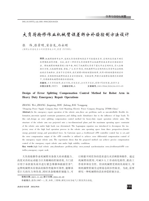
3x=D1 +D2 sin谆2 +D3 sin谆3

y＝0
（1）

z=D1+D2 cos谆2+D3cos谆3
观察图1 可发现，抢修机械臂在 xoy 二维平面
内存在 4 条投影边界曲线，分别为 P1 P2、P1 P4、P2 P3、 P3 P4，4 条边界曲线的交点为 P1（x1，y1）、P2（x2，y2）、 P3（x3，y3）、P4（x4，y4），通过计算 4 个圆弧半径的最小值，可以确定机械臂在满足各种位姿要求的前提
N
移 Eqቤተ መጻሕፍቲ ባይዱ= Enq
（7）
n＝１
（3）机械臂广义力分量抢修机械臂作业过程中，由于机械臂的弯曲，中心弹性杠杆以及杠杆驱动线呈同一角度弯曲，设 A f 、Al 分别为机械臂连杆作业过程中雅可比矩阵以及驱动线雅可比矩阵[7]，则机械臂的广义力分量为
（Dongying Power Supply Company，State Grid Shandong Electric Power Company，Dongying 257000，China） Abstract：In the emergency repair operation of the robotic arm，there are problems such as uncontrollable flexible de鄄 formation，uncertain spatial constraint parameters，and sliding mode disturbance due to the influence of large loads. To this end，design an error splitting compensation control method for heavy鄄duty repair operation robotic arms. The structure of the robotic arm was projected onto a two鄄dimensional plane，and the maximum operating space constraint of the robotic arm under high loads was determined. The Lagrangian equation was introduced to decompose the tra鄄 jectory error of the high load operation process in the robotic arm operating space from three perspectives：kinetic energy，potential energy，and generalized force. In Cartesian space，a feedforward +PD controller control law is set，and the error compensation output of the +PD controller is utilized to achieve error differential compensation control of the emergency repair robotic arm. The experiment shows that the proposed method can achieve precise compensation control of the emergency repair robotic arm under high stability conditions. Key words：high load robotic arm；disturbance problem；delay error；normal synchronization error；feedforward+PD con鄄 troller；emergency repair work

机器人应用手册说明书

for assembly 129-31 for handling 118-19 for machining 171-3 for spray painting 188-96 for welding 151, 163-6
see also behaviour charge-coupled devices 81-2 Cincinnati Milacron robots 2
7-8,20-1,112 automobile industry see leak
testing; spot welding; spray painting axes end-effector 30 extra 29, 119 multiple 6-7
behaviour characteristics long-term 43-6 stationary 46-7 see also aberrant behaviour
gripper 67 performance testing and 43,
44 see also direct drives; electric
drives; hydraulic drives; pneumatic drives duplication of joints 30 dynamic camera positioning 84-5 dynamic control 33-4 dynamic performance 49
fail-safe brakes 161 laying-up of composites 208-
9 machining 174,175 water jet cutting 206 clamping grippers 61-71 classification of robot systems

1、下载文档前请自行甄别文档内容的完整性，平台不提供额外的编辑、内容补充、找答案等附加服务。
2、"仅部分预览"的文档,不可在线预览部分如存在完整性等问题,可反馈申请退款(可完整预览的文档不适用该条件!)。
3、如文档侵犯您的权益，请联系客服反馈,我们会尽快为您处理(人工客服工作时间：9:00-18:30)。

Feedback Control For Robot Formation Maneuvers
Brett J. Young Jonathan R. Lawton Randal W. Beard Electrical and Computer Engineering Department Brigham Young University
xhid (t) = xc (t) + Di (t) cos( (t) + 0i ) (11) yhid (t) = yc (t) + Di (t) sin( (t) + 0i ); (12) where Di (t) is the relative distance from the desired
over say spacecraft is that they are easier to test and less expensive to maintain. Also introducing feedback from the followers to the leader seems natural since the leader should not move too fast or too slow for the followers. The outline of the paper is as follows: in Section 2 we introduce the robot model. In Section 3 we introduce the type of formation maneuvers we will consider. In பைடு நூலகம்ection 4 we try to motivate using a virtual leader over a real leader for leader-follower. In Section 5 we present virtual leader-follower schemes. We rst show how the traditional leader follower works for a group of robots. Then we introduce the novel concept of having the followers send feedback to the leader. Finally, in Section 6 we present hardware results for the virtual leader follower schemes with and without feedback from the followers to the leader.
35
30
25
20
15
xh = x + L cos( ) yh = y + L sin( ):
Then xh , yh are given by:
(6) (7) (8)
10
−10
−5
0
5
10
15
20
xh = R( ) yh
F M L J
F M L J
? L!2 : + v!
Figure 1: The template evolves according to some dynamics.
1 Introduction
Moving a group of agents in formation has received a fair amount of attention in the literature. There are dozens of papers which look at the problem. Many take a biological approach 1] in which they try to mimic birds ocking or herds migrating. However most fall under either a leader-follower type scheme or an emergent behavior scheme. In 2] a leader-follower scheme is presented for mobile robots. The leader is supposed to have some trajectory (possibly given by a path planner) and the other robots track the leader. As a variation on this scheme, a robot may track the average position of his two closest neighbors. Another type of leader follower scheme is presented in 3]. Here, the leader is a virtual structure. The structure is least squares t to the robots, then the structure propagates and the robots follow in an open loop fashion and the process is repeated. Virtual structures are also used in path planning or tracking which can be thought of as one robot moving in formation 4]. The idea of a virtual leader is also introduced in 5] for a group of spacecraft ying in formation. Behavioral approaches are common for robots. An example for robots can be found in 1]. The purpose of this paper is to extend some of the explicit closed loop leader-follower formation control ideas developed for spacecraft to Hilare-type mobile robots and to introduce feedback from the followers to the leader for improved robustness. There are several reasons for doing this. One reason for using robots 1
Letting F, and be given by:
L!2 = ?v! + R(? ) ux : uy xh = ux : uy yh
(9) (10)
This reduces to:
ith location for the robot and the virtual center and where 0i (t) is the angle relative to the template center. For example, to perform a translation let,
(2) (3) (4)
mv = F _ J! = ; _
(5) where m is the mass, J the inertia, F is force and the torque. Equations (1) and (2) restrict translational motion of the robot to be in the direction perpendicular to the drive axis, known as the non-holonomic constraint. Combining this with Equation (3), the robot
3 Elementary Formation Maneuvers
The idea of Elementary Formation Maneuvers stems from those used in satellites 5]. With just a few simple maneuvers, most any desired form of group maneuvers which preserve formation shape can be achieved. These maneuvers could be thought of as a kernel or basis for most other types of formation maneuvers which preserve formation shapes. The basic maneuvers are: Translations Expansions/Contractions Rotations. Performing Elementary Formation Maneuvers for leader follower is fairly straight forward. The leader moves in the desired direction and the desired trajectories for the followers are rigidly connected to the leader. For the virtual leader-follower the maneuvers may look like Figure 1. The virtual leader has a center with a speci c orientation which shall be denoted (xc (t),yc (t), c (t)). The desired hand position of the ith robot with respect to the center is given by: