Exploiting Covariate Similarity in Sparse Regression via the Pairwise Elastic Net
相似度的计算
相似度计算1相似度的计算简介关于相似度的计算,现有的几种基本方法都是基于向量(Vector)的,其实也就是计算两个向量的距离,距离越近相似度越大。
在推荐的场景中,在用户-物品偏好的二维矩阵中,我们可以将一个用户对所有物品的偏好作为一个向量来计算用户之间的相似度,或者将所有用户对某个物品的偏好作为一个向量来计算物品之间的相似度。
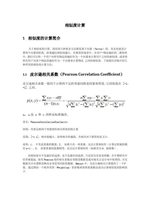
下面我们详细介绍几种常用的相似度计算方法:1.1皮尔逊相关系数(Pearson Correlation Coefficient)皮尔逊相关系数一般用于计算两个定距变量间联系的紧密程度,它的取值在 [-1,+1] 之间。
s x , sy是 x 和 y 的样品标准偏差。
类名:PearsonCorrelationSimilarity原理:用来反映两个变量线性相关程度的统计量范围:[-1,1],绝对值越大,说明相关性越强,负相关对于推荐的意义小。
说明:1、不考虑重叠的数量;2、如果只有一项重叠,无法计算相似性(计算过程被除数有n-1);3、如果重叠的值都相等,也无法计算相似性(标准差为0,做除数)。
该相似度并不是最好的选择,也不是最坏的选择,只是因为其容易理解,在早期研究中经常被提起。
使用Pearson线性相关系数必须假设数据是成对地从正态分布中取得的,并且数据至少在逻辑范畴内必须是等间距的数据。
Mahout中,为皮尔森相关计算提供了一个扩展,通过增加一个枚举类型(Weighting)的参数来使得重叠数也成为计算相似度的影响因子。
1.2欧几里德距离(Euclidean Distance)最初用于计算欧几里德空间中两个点的距离,假设 x,y 是 n 维空间的两个点,它们之间的欧几里德距离是:可以看出,当 n=2 时,欧几里德距离就是平面上两个点的距离。
当用欧几里德距离表示相似度,一般采用以下公式进行转换:距离越小,相似度越大。
类名:EuclideanDistanceSimilarity原理:利用欧式距离d定义的相似度s,s=1 / (1+d)。
英文论文写作中一些可能用到的词汇
英⽂论⽂写作中⼀些可能⽤到的词汇英⽂论⽂写作过程中总是被⾃⼰可怜的词汇量击败, 所以我打算在这⾥记录⼀些在阅读论⽂过程中见到的⼀些⾃⼰不曾见过的词句或⽤法。
这些词句查词典都很容易查到,但是只有带⼊论⽂原⽂中才能体会内涵。
毕竟原⽂和译⽂中间总是存在⼀条看不见的思想鸿沟。
形容词1. vanilla: adj. 普通的, 寻常的, 毫⽆特⾊的. ordinary; not special in any way.2. crucial: adj. ⾄关重要的, 关键性的.3. parsimonious:adj. 悭吝的, 吝啬的, ⼩⽓的.e.g. Due to the underlying hyperbolic geometry, this allows us to learn parsimonious representations of symbolic data by simultaneously capturing hierarchy and similarity.4. diverse: adj. 不同的, 相异的, 多种多样的, 形形⾊⾊的.5. intriguing: adj. ⾮常有趣的, 引⼈⼊胜的; 神秘的. *intrigue: v. 激起…的兴趣, 引发…的好奇⼼; 秘密策划(加害他⼈), 密谋.e.g. The results of this paper carry several intriguing implications.6. intimate: adj. 亲密的; 密切的. v.透露; (间接)表⽰, 暗⽰.e.g. The above problems are intimately linked to machine learning on graphs.7. akin: adj. 类似的, 同族的, 相似的.e.g. Akin to GNN, in LOCAL a graph plays a double role: ...8. abundant: adj. ⼤量的, 丰盛的, 充裕的.9. prone: adj. 有做(坏事)的倾向; 易于遭受…的; 俯卧的.e.g. It is thus prone to oversmoothing when convolutions are applied repeatedly.10.concrete: adj. 混凝⼟制的; 确实的, 具体的(⽽⾮想象或猜测的); 有形的; 实在的.e.g. ... as a concrete example ...e.g. More concretely, HGCN applies the Euclidean non-linear activation in...11. plausible: adj. 有道理的; 可信的; 巧⾔令⾊的, 花⾔巧语的.e.g. ... this interpretation may be a plausible explanation of the success of the recently introduced methods.12. ubiquitous: adj. 似乎⽆所不在的;⼗分普遍的.e.g. While these higher-order interac- tions are ubiquitous, an evaluation of the basic properties and organizational principles in such systems is missing.13. disparate: adj. 由不同的⼈(或事物)组成的;迥然不同的;⽆法⽐较的.e.g. These seemingly disparate types of data have something in common: ...14. profound: adj. 巨⼤的; 深切的, 深远的; 知识渊博的; 理解深刻的;深邃的, 艰深的; ⽞奥的.e.g. This has profound consequences for network models of relational data — a cornerstone in the interdisciplinary study of complex systems.15. blurry: adj. 模糊不清的.e.g. When applying these estimators to solve (2), the line between the critic and the encoders $g_1, g_2$ can be blurry.16. amenable: adj. 顺从的; 顺服的; 可⽤某种⽅式处理的.e.g. Ou et al. utilize sparse generalized SVD to generate a graph embedding, HOPE, from a similarity matrix amenableto de- composition into two sparse proximity matrices.17. elaborate: adj. 复杂的;详尽的;精⼼制作的 v.详尽阐述;详细描述;详细制订;精⼼制作e.g. Topic Modeling for Graphs also requires elaborate effort, as graphs are relational while documents are indepen- dent samples.18. pivotal: adj. 关键性的;核⼼的e.g. To ensure the stabilities of complex systems is of pivotal significance toward reliable and better service providing.19. eminent: adj. 卓越的,著名的,显赫的;⾮凡的;杰出的e.g. To circumvent those defects, theoretical studies eminently represented by percolation theories appeared.20. indispensable: adj. 不可或缺的;必不可少的 n. 不可缺少的⼈或物e.g. However, little attention is paid to multipartite networks, which are an indispensable part of complex networks.21. post-hoc: adj. 事后的e.g. Post-hoc explainability typically considers the question “Why the GNN predictor made certain prediction?”.22. prevalent: adj. 流⾏的;盛⾏的;普遍存在的e.g. A prevalent solution is building an explainer model to conduct feature attribution23. salient: adj. 最重要的;显著的;突出的. n. 凸⾓;[建]突出部;<军>进攻或防卫阵地的突出部分e.g. It decomposes the prediction into the contributions of the input features, which redistributes the probability of features according to their importance and sample the salient features as an explanatory subgraph.24. rigorous: adj. 严格缜密的;严格的;谨慎的;细致的;彻底的;严厉的e.g. To inspect the OOD effect rigorously, we take a causal look at the evaluation process with a Structural Causal Model.25. substantial: adj. ⼤量的;价值巨⼤的;重⼤的;⼤⽽坚固的;结实的;牢固的. substantially: adv. ⾮常;⼤⼤地;基本上;⼤体上;总的来说26. cogent: adj. 有说服⼒的;令⼈信服的e.g. The explanatory subgraph $G_s$ emphasizes tokens like “weak” and relations like “n’t→funny”, which is cogent according to human knowledge.27. succinct: adj. 简练的;简洁的 succinctly: adv. 简⽽⾔之,简明扼要地28. concrete: adj. 混凝⼟制的;确实的,具体的(⽽⾮想象或猜测的);有形的;实在的 concretely: adv. 具体地;具体;具体的;有形地29. predominant:adj. 主要的;主导的;显著的;明显的;盛⾏的;占优势的动词1. mitigate: v. 减轻, 缓和. (反 enforce)e.g. In this work, we focus on mitigating this problem for a certain class of symbolic data.2. corroborate: v. [VN] [often passive] (formal) 证实, 确证.e.g. This is corroborated by our experiments on real-world graph.3. endeavor: n./v. 努⼒, 尽⼒, 企图, 试图.e.g. It encourages us to continue the endeavor in applying principles mathematics and theory in successful deployment of deep learning.4. augment: v. 增加, 提⾼, 扩⼤. n. 增加, 补充物.e.g. We also augment the graph with geographic information (longitude, latitude and altitude), and GDP of the country where the airport belongs to.5. constitute: v. (被认为或看做)是, 被算作; 组成, 构成; (合法或正式地)成⽴, 设⽴.6. abide: v. 接受, 遵照(规则, 决定, 劝告); 逗留, 停留.e.g. Training a graph classifier entails identifying what constitutes a class, i.e., finding properties shared by graphs in one class but not the other, and then deciding whether new graphs abide to said learned properties.7. entail: v. 牵涉; 需要; 使必要. to involve sth that cannot be avoided.e.g. Due to the recursive definition of the Chebyshev polynomials, the computation of the filter $g_α(\Delta)f$ entails applying the Laplacian $r$ times, resulting cal operator affecting only 1-hop neighbors of a vertex and in $O(rn)$ operations.8. encompass: v. 包含, 包括, 涉及(⼤量事物); 包围, 围绕, 围住.e.g. This model is chosen as it is sufficiently general to encompass several state-of-the-art networks.e.g. The k-cycle detection problem entails determining if G contains a k-cycle.9. reveal: v. 揭⽰, 显⽰, 透露, 显出, 露出, 展⽰.10. bestow: v. 将(…)给予, 授予, 献给.e.g. Aiming to bestow GCNs with theoretical guarantees, one promising research direction is to study graph scattering transforms (GSTs).11. alleviate: v. 减轻, 缓和, 缓解.12. investigate: v. 侦查(某事), 调查(某⼈), 研究, 调查.e.g. The sensitivity of pGST to random and localized noise is also investigated.13. fuse: v. (使)融合, 熔接, 结合; (使)熔化, (使保险丝熔断⽽)停⽌⼯作.e.g. We then fuse the topological embeddings with the initial node features into the initial query representations using a query network$f_q$ implemented as a two-layer feed-forward neural network.14. magnify: v. 放⼤, 扩⼤; 增强; 夸⼤(重要性或严重性); 夸张.e.g. ..., adding more layers also leads to more parameters which magnify the potential of overfitting.15. circumvent: v. 设法回避, 规避; 绕过, 绕⾏.e.g. To circumvent the issue and fulfill both goals simultaneously, we can add a negative term...16. excel: v. 擅长, 善于; 突出; 胜过平时.e.g. Nevertheless, these methods have been repeatedly shown to excel in practice.17. exploit: v. 利⽤(…为⾃⼰谋利); 剥削, 压榨; 运⽤, 利⽤; 发挥.e.g. In time series and high-dimensional modeling, approaches that use next step prediction exploit the local smoothness of the signal.18. regulate: v. (⽤规则条例)约束, 控制, 管理; 调节, 控制(速度、压⼒、温度等).e.g. ... where $b >0$ is a parameter regulating the probability of this event.19. necessitate: v. 使成为必要.e.g. Combinatorial models reproduce many-body interactions, which appear in many systems and necessitate higher-order models that capture information beyond pairwise interactions.20. portray:描绘, 描画, 描写; 将…描写成; 给⼈以某种印象; 表现; 扮演(某⾓⾊).e.g. Considering pairwise interactions, a standard network model would portray the link topology of the underlying system as shown in Fig. 2b.21. warrant: v. 使有必要; 使正当; 使恰当. n. 执⾏令; 授权令; (接受款项、服务等的)凭单, 许可证; (做某事的)正当理由, 依据.e.g. Besides statistical methods that can be used to detect correlations that warrant higher-order models, ... (除了可以⽤来检测⽀持⾼阶模型的相关性的统计⽅法外, ...)22. justify: v. 证明…正确(或正当、有理); 对…作出解释; 为…辩解(或辩护); 调整使全⾏排满; 使每⾏排齐.e.g. ..., they also come with the assumption of transitive, Markovian paths, which is not justified in many real systems.23. hinder:v. 阻碍; 妨碍; 阻挡. (反 foster: v. 促进; 助长; 培养; ⿎励; 代养, 抚育, 照料(他⼈⼦⼥⼀段时间))e.g. The eigenvalues and eigenvectors of these matrix operators capture how the topology of a system influences the efficiency of diffusion and propagation processes, whether it enforces or mitigates the stability of dynamical systems, or if it hinders or fosters collective dynamics.24. instantiate:v. 例⽰;⽤具体例⼦说明.e.g. To learn the representation we instantiate (2) and split each input MNIST image into two parts ...25. favor:v. 赞同;喜爱, 偏爱; 有利于, 便于. n. 喜爱, 宠爱, 好感, 赞同; 偏袒, 偏爱; 善⾏, 恩惠.26. attenuate: v. 使减弱; 使降低效⼒.e.g. It therefore seems that the bounds we consider favor hard-to-invert encoders, which heavily attenuate part of the noise, over well conditioned encoders.27. elucidate:v. 阐明; 解释; 说明.e.g. Secondly, it elucidates the importance of appropriately choosing the negative samples, which is indeed a critical component in deep metric learning based on triplet losses.28. violate: v. 违反, 违犯, 违背(法律、协议等); 侵犯(隐私等); 使⼈不得安宁; 搅扰; 亵渎, 污损(神圣之地).e.g. Negative samples are obtained by patches from different images as well as patches from the same image, violating the independence assumption.29. compel:v. 强迫, 迫使; 使必须; 引起(反应).30. gauge: v. 判定, 判断(尤指⼈的感情或态度); (⽤仪器)测量, 估计, 估算. n. 测量仪器(或仪表);计量器;宽度;厚度;(枪管的)⼝径e.g. Yet this hyperparameter-tuned approach raises a cubic worst-case space complexity and compels the user to traverse several feature sets and gauge the one that attains the best performance in the downstream task.31. depict: v. 描绘, 描画; 描写, 描述; 刻画.e.g. As they depict different aspects of a node, it would take elaborate designs of graph convolutions such that each set of features would act as a complement to the other.32. sketch: n. 素描;速写;草图;幽默短剧;⼩品;简报;概述 v. 画素描;画速写;概述;简述e.g. Next we sketch how to apply these insights to learning topic models.33. underscore:v. 在…下⾯划线;强调;着重说明 n.下划线e.g. Moreover, the walk-topic distributions generated by Graph Anchor LDA are indeed sharper than those by ordinary LDA, underscoring the need for selecting anchors.34. disclose: v. 揭露;透露;泄露;使显露;使暴露e.g. Another drawback lies in their unexplainable nature, i.e., they cannot disclose the sciences beneath network dynamics.35. coincide: v. 同时发⽣;相同;相符;极为类似;相接;相交;同位;位置重合;重叠e.g. The simulation results coincide quite well with the theoretical results.36. inspect: v. 检查;查看;审视;视察 to look closely at sth/sb, especially to check that everything is as it should be名词1. capacity: n. 容量, 容积, 容纳能⼒; 领悟(或理解、办事)能⼒; 职位, 职责.e.g. This paper studies theoretically the computational capacity limits of graph neural networks (GNN) falling within the message-passing framework of Gilmer et al. (2017).2. implication: n. 可能的影响(或作⽤、结果); 含意, 暗指; (被)牵连, 牵涉.e.g. Section 4 analyses the implications of restricting the depth $d$ and width $w$ of GNN that do not use a readout function.3. trade-off:(在需要⽽⼜相互对⽴的两者间的)权衡, 协调.e.g. This reveals a direct trade-off between the depth and width of a graph neural network.4. cornerstone:n. 基⽯; 最重要部分; 基础; 柱⽯.5. umbrella: n. 伞; 综合体; 总体, 整体; 保护, 庇护(体系).e.g. Community detection is an umbrella term for a large number of algorithms that group nodes into distinct modules to simplify and highlight essential structures in the network topology.6. folklore:n. 民间传统, 民俗; 民间传说.e.g. It is folklore knowledge that maximizing MI does not necessarily lead to useful representations.7. impediment:n. 妨碍,阻碍,障碍; ⼝吃.e.g. While a recent approach overcomes this impediment, it results in poor quality in prediction tasks due to its linear nature.8. obstacle:n. 障碍;阻碍; 绊脚⽯; 障碍物; 障碍栅栏.e.g. However, several major obstacles stand in our path towards leveraging topic modeling of structural patterns to enhance GCNs.9. vicinity:n. 周围地区; 邻近地区; 附近.e.g. The traits with which they engage are those that are performed in their vicinity.10. demerit: n. 过失,缺点,短处; (学校给学⽣记的)过失分e.g. However, their principal demerit is that their implementations are time-consuming when the studied network is large in size. Another介/副/连词1. notwithstanding:prep. 虽然;尽管 adv. 尽管如此.e.g. Notwithstanding this fundamental problem, the negative sampling strategy is often treated as a design choice.2. albeit: conj. 尽管;虽然e.g. Such methods rely on an implicit, albeit rigid, notion of node neighborhood; yet this one-size-fits-all approach cannot grapple with the diversity of real-world networks and applications.3. Hitherto:adv. 迄今;直到某时e.g. Hitherto, tremendous endeavors have been made by researchers to gauge the robustness of complex networks in face of perturbations.短语1.in a nutshell: 概括地说, 简⾔之, ⼀⾔以蔽之.e.g. In a nutshell, GNN are shown to be universal if four strong conditions are met: ...2. counter-intuitively: 反直觉地.3. on-the-fly:动态的(地), 运⾏中的(地).4. shed light on/into:揭⽰, 揭露; 阐明; 解释; 将…弄明⽩; 照亮.e.g. These contemporary works shed light into the stability and generalization capabilities of GCNs.e.g. Discovering roles and communities in networks can shed light on numerous graph mining tasks such as ...5. boil down to: 重点是; 将…归结为.e.g. These aforementioned works usually boil down to a general classification task, where the model is learnt on a training set and selected by checking a validation set.6. for the sake of:为了.e.g. The local structures anchored around each node as well as the attributes of nodes therein are jointly encoded with graph convolution for the sake of high-level feature extraction.7. dates back to:追溯到.e.g. The usual problem setup dates back at least to Becker and Hinton (1992).8. carry out:实施, 执⾏, 实⾏.e.g. We carry out extensive ablation studies and sensi- tivity analysis to show the effectiveness of the proposed functional time encoding and TGAT-layer.9. lay beyond the reach of:...能⼒达不到e.g. They provide us with information on higher-order dependencies between the components of a system, which lay beyond the reach of models that exclusively capture pairwise links.10. account for: ( 数量或⽐例上)占; 导致, 解释(某种事实或情况); 解释, 说明(某事); (某⼈)对(⾏动、政策等)负有责任; 将(钱款)列⼊(预算).e.g. Multilayer models account for the fact that many real complex systems exhibit multiple types of interactions.11. along with: 除某物以外; 随同…⼀起, 跟…⼀起.e.g. Along with giving us the ability to reason about topological features including community structures or node centralities, network science enables us to understand how the topology of a system influences dynamical processes, and thus its function.12. dates back to:可追溯到.e.g. The usual problem setup dates back at least to Becker and Hinton (1992) and can conceptually be described as follows: ...13. to this end:为此⽬的;为此计;为了达到这个⽬标.e.g. To this end, we consider a simple setup of learning a representation of the top half of MNIST handwritten digit images.14. Unless stated otherwise:除⾮另有说明.e.g. Unless stated otherwise, we use a bilinear critic $f(x, y) = x^TWy$, set the batch size to $128$ and the learning rate to $10^{−4}$.15. As a reference point:作为参照.e.g. As a reference point, the linear classification accuracy from pixels drops to about 84% due to the added noise.16. through the lens of:透过镜头. (以...视⾓)e.g. There are (at least) two immediate benefits of viewing recent representation learning methods based on MI estimators through the lens of metric learning.17. in accordance with:符合;依照;和…⼀致.e.g. The metric learning view seems hence in better accordance with the observations from Section 3.2 than the MI view.It can be shown that the anchors selected by our Graph Anchor LDA are not only indicative of “topics” but are also in accordance with the actual graph structures.18. be akin to:近似, 类似, 类似于.e.g. Thus, our learning model is akin to complex contagion dynamics.19. to name a few:仅举⼏例;举⼏个来说.e.g. Multitasking, multidisciplinary work and multi-authored works, to name a few, are ingrained in the fabric of science culture and certainly multi-multi is expected in order to succeed and move up the scientific ranks.20. a handful of:⼀把;⼀⼩撮;少数e.g. A handful of empirical work has investigated the robustness of complex networks at the community level.21. wreak havoc: 破坏;肆虐;严重破坏;造成破坏;浩劫e.g. Failures on one network could elicit failures on its coupled networks, i.e., networks with which the focal network interacts, and eventually those failures would wreak havoc on the entire network.22. apart from: 除了e.g. We further posit that apart from node $a$ node $b$ has $k$ neighboring nodes.。
同义词判别模型
同义词判别模型同义词判别模型是一种自然语言处理(NLP)技术,旨在识别和判断语言中的同义词。
同义词是那些意思相同或非常接近的词汇,比如“快速”和“迅速”,在很多情况下可以互换使用而不改变句子的基本含义。
同义词判别模型的开发对于机器翻译、文本摘要、信息检索、问答系统等众多NLP 应用至关重要。
基本原理同义词判别模型基于这样一个假设:语境相似的词语往往具有相似的含义。
因此,这些模型通常依赖于大量的语料库数据来学习单词之间的语义关系。
通过分析单词在不同语境中的共现模式,模型能够捕捉到它们之间的语义相似度。
关键技术和方法1. 向量空间模型:将单词表示为高维空间中的向量,其中每一维对应一个特定的语境特征。
通过计算向量之间的余弦相似度,可以估计单词之间的语义相似性。
2. 词嵌入模型:通过训练将单词映射到连续的向量空间中,使得语义上相近的单词在向量空间中也彼此靠近。
3. 深度学习模型:例如循环神经网络、长短期记忆网络和Transformer架构,它们能够考虑上下文信息,并生成更为精确的词义表示。
4. 知识图谱和本体论:利用结构化的知识库,这些库包含了大量的词汇及其相互之间的关系,可以用来推断词汇间的同义关系。
挑战与问题开发同义词判别模型面临诸多挑战,包括词义消歧、多义性处理、跨语言差异等。
例如,许多单词在不同的语境下有不同的意义,模型需要能够准确地识别出这些不同的语境。
此外,由于文化和语言习惯的差异,不同语言之间的同义词可能没有直接的对应关系。
应用同义词判别模型的应用非常广泛,包括但不限于:- 机器翻译:选择最合适的目标语言词汇来翻译源语言中的单词。
- 搜索引擎优化:理解查询中的同义词,以返回更相关的搜索结果。
- **自动文摘和文本生成**:在不改变原意的情况下,使用多样化的词汇来创建流畅的文本。
- 问答系统:理解用户提问的不同表达方式,提供准确的答案。
发展趋势随着深度学习技术的发展,预训练语言模型(如BERT和其变体)在同义词判别任务上取得了显著进展。
贝叶斯网络的近似推断方法

贝叶斯网络的近似推断方法贝叶斯网络是一种用概率图模型来表示随机变量之间依赖关系的工具。
在实际应用中,我们常常需要对贝叶斯网络进行推断,即给定部分变量的取值,推断其他变量的分布。
然而,对于复杂的贝叶斯网络,精确推断往往是不可行的,因此需要采用近似推断方法。
马尔科夫链蒙特卡洛方法(MCMC)是一种常用的近似推断方法。
它通过构建马尔科夫链,利用马尔科夫链的平稳分布来逼近目标分布。
MCMC方法的优点在于能够处理任意形状的分布,但缺点是收敛速度慢,对参数敏感,并且需要大量的样本。
变分推断是另一种常用的近似推断方法。
它通过寻找一个与目标分布“最接近”的分布来逼近目标分布。
变分推断的优点在于收敛速度快,对参数不敏感,但缺点是只能处理一部分的分布形状。
在近年来,由于深度学习的发展,基于神经网络的近似推断方法也越来越受到关注。
变分自动编码器(VAE)就是一种基于神经网络的近似推断方法。
它通过将变分推断和神经网络结合起来,可以处理更加复杂的分布形状。
除了上述方法外,还有一些其他的近似推断方法,比如重要性采样、拉普拉斯近似等。
这些方法各有优缺点,适用于不同的问题和场景。
在实际应用中,选择合适的近似推断方法是非常重要的。
一方面,要考虑到目标分布的形状,是否能够用某种近似推断方法来逼近;另一方面,也要考虑到计算资源和时间的限制,选择合适的方法来平衡计算效率和推断准确度。
总的来说,贝叶斯网络的近似推断方法是一个非常有挑战性的课题,需要综合考虑概率统计、优化方法和计算机科学等多个领域的知识。
随着人工智能和机器学习的不断发展,相信在未来会有更多更好的近似推断方法出现,为贝叶斯网络的应用提供更加强大的支持。
机器学习与数据挖掘笔试面试题

Why do we combine multiple trees? What is Random Forest? Why would you prefer it to SVM? Logistic regression: Link to Logistic regression Here's a nice tutorial What is logistic regression? How do we train a logistic regression model? How do we interpret its coefficients? Support Vector Machines A tutorial on SVM can be found and What is the maximal margin classifier? How this margin can be achieved and why is it beneficial? How do we train SVM? What about hard SVM and soft SVM? What is a kernel? Explain the Kernel trick Which kernels do you know? How to choose a kernel? Neural Networks Here's a link to on Coursera What is an Artificial Neural Network? How to train an ANN? What is back propagation? How does a neural network with three layers (one input layer, one inner layer and one output layer) compare to a logistic regression? What is deep learning? What is CNN (Convolution Neural Network) or RNN (Recurrent Neural Network)? Other models: What other models do you know? How can we use Naive Bayes classifier for categorical features? What if some features are numerical? Tradeoffs between different types of classification models. How to choose the best one? Compare logistic regression with decision trees and neural networks. and What is Regularization? Which problem does Regularization try to solve? Ans. used to address the overfitting problem, it penalizes your loss function by adding a multiple of an L1 (LASSO) or an L2 (Ridge) norm of your weights vector w (it is the vector of the learned parameters in your linear regression). What does it mean (practically) for a design matrix to be "ill-conditioned"? When might you want to use ridge regression instead of traditional linear regression? What is the difference between the L1 and L2 regularization? Why (geometrically) does LASSO produce solutions with zero-valued coefficients (as opposed to ridge)? and What is the purpose of dimensionality reduction and why do we need it? Are dimensionality reduction techniques supervised or not? Are all of them are (un)supervised? What ways of reducing dimensionality do you know? Is feature selection a dimensionality reduction technique? What is the difference between feature selection and feature extraction? Is it beneficial to perform dimensionality reduction before fitting an SVM? Why or why not? and Why do you need to use cluster analysis? Give examples of some cluster analysis methods? Differentiate between partitioning method and hierarchical methods. Explain K-Means and its objective? How do you select K for K-Means?
应用CARS和SPA算法对草莓SSC含量NIR光谱预测模型中变量及样本筛选
0 . 3 4 8 4和 3 . 3 2 7 8。
, R MS E P和 R P D分别为 0 . 9 0 9 7 ,
关键词
变量筛选 ; 样本筛选 ; 近红外光谱 ; 草莓 ;可溶性 固形物
所有波长点都有用 ;另一方 面 , 部分 波长之 间也存在 较为严
重 的共线性 。目前的研究已经证 明冗 余信息 的存在 能够削弱 模 型的预测性 能和稳 定性 _ 3 ] 。因此 , 在 利用 近红 外光 谱对 农 产品无损检测 时,需要 进行 无信 息变量 消除 和变量优 选 。 在众 多变量选择 的算法 中 , 蒙特卡罗无信息变量消除 ( Mo n t e
第3 5 卷 , 第2 期
2 0 1 5年 2月
光
谱
学
与
光
谱
分
析
S p e c t r o s c o p y a n d S p e c t r a l An a l y s i s
Vo 1 . 3 5 , No . 2 , p p 3 7 2 — 3 7 8 Fe b r u a r y ,2 0 1 5
有“ 水果 皇后 ” 的美称 。 开展基于草莓 内部 品质的快速 检测分 级技术研究具有重要意义 。 本研究 中将 C A R S变量选 择方法
影算法 ( s u c c e s s i v e p r o j e c t i o n s a l g o r i t h m,s P A) 是两种分别在
个关键变量 。 为 了验证 C R S算法的性能 , A 蒙特卡罗无信息变量消除 MC - UV E和连续投影算法 S P A用于 比 较研究 。C R S算法在 消除无信息变量 的同时可 以对共线 性信息进 行去 除。同样 , A 为 了评估 S P A算 法在特 征样本选择 中的性能 ,经典的 Ke n n a r d - S t o n e 算法也用于 比较分析 。S P A算法能够用于校正 集特征样本 的优
与马尔可夫链蒙特卡洛法类似的方法
与马尔可夫链蒙特卡洛法类似的方法马尔可夫链蒙特卡洛法(Markov Chain Monte Carlo, MCMC)是一种用于估计复杂概率分布的方法,广泛应用于统计学、机器学习和计算机视觉等领域。
然而,除了MCMC之外,还存在一些与之类似的方法,本文将介绍其中的几种。
1. 重要性采样(Importance Sampling)重要性采样是一种基于蒙特卡洛方法的统计估计方法,用于计算一个概率分布的期望值。
其核心思想是通过从一个已知的简单分布中采样,来估计一个复杂的目标分布的期望值。
与MCMC类似,重要性采样也利用随机采样的方式来估计目标分布的特征。
然而,与MCMC不同的是,重要性采样不需要满足马尔可夫链的平稳性质,因此在某些情况下更加高效。
2. 随机优化方法(Stochastic Optimization)随机优化方法是一类基于随机采样的优化算法,用于解决无法直接求解的优化问题。
与MCMC类似,随机优化方法也利用随机采样的方式来估计优化目标函数的值。
不同的是,随机优化方法更加关注优化问题本身,通过随机采样来探索优化空间,并更新优化参数以寻找最优解。
在大规模数据和高维优化问题中,随机优化方法通常比传统的优化算法更加高效。
3. 变分贝叶斯方法(Variational Bayesian Methods)变分贝叶斯方法是一种基于变分推断的概率建模方法,用于近似推断复杂的概率分布。
与MCMC类似,变分贝叶斯方法也通过随机采样的方式来近似复杂的后验分布。
然而,变分贝叶斯方法更加注重推断过程的优化,通过引入一个近似分布来近似后验分布,并通过优化近似分布的参数来逼近真实后验分布。
相比于MCMC,变分贝叶斯方法通常具有更快的收敛速度和更好的可解释性。
4. 重要性抽样平均(Importance Sampling Average)重要性抽样平均是一种基于随机抽样的估计方法,用于计算概率分布的平均值。
与MCMC类似,重要性抽样平均也利用随机采样的方式来估计目标分布的特征。
贝叶斯网络的近似推断方法(五)
贝叶斯网络是一种用来描述随机变量之间依赖关系的图模型,也是一种用来进行概率推断的工具。
在实际应用中,贝叶斯网络可以帮助我们对未知变量进行推断,从而做出更加合理的决策。
然而,精确的贝叶斯推断通常需要计算复杂的概率分布,这在实际问题中往往是不可行的。
因此,近似推断方法成为了贝叶斯网络研究的重要内容之一。
一、蒙特卡洛方法蒙特卡洛方法是一种常见的近似推断方法。
它通过从概率分布中抽取大量的样本来近似计算分布的期望值。
在贝叶斯网络中,蒙特卡洛方法可以用来对后验分布进行近似推断。
具体来说,我们可以通过抽取大量的样本来近似计算后验概率分布,从而得到对未知变量的推断结果。
蒙特卡洛方法的优点是简单易行,而且在一定条件下可以得到较为精确的近似结果。
但是,它也存在着计算量大、收敛速度慢等缺点,特别是在高维问题中往往难以有效应用。
二、变分推断方法变分推断方法是另一种常见的近似推断方法。
它通过寻找一个与真实后验分布相近的分布来进行推断。
在贝叶斯网络中,变分推断方法可以通过最大化一个变分下界来近似计算后验分布。
具体来说,我们可以假设一个参数化的分布族,然后寻找一个参数使得该分布在KL散度意义下与真实后验分布最为接近。
变分推断方法的优点是可以通过参数化的方式来近似计算后验分布,从而在一定程度上减少计算量。
但是,它也存在着对分布族的选择敏感、局部最优解等问题。
三、马尔科夫链蒙特卡洛方法马尔科夫链蒙特卡洛方法是一种结合了蒙特卡洛方法和马尔科夫链的近似推断方法。
它通过构建一个转移核函数来对后验分布进行采样,从而得到对未知变量的推断结果。
在贝叶斯网络中,马尔科夫链蒙特卡洛方法可以用来对后验分布进行采样。
具体来说,我们可以构建一个马尔科夫链,使得其平稳分布为真实后验分布,然后通过该链进行采样。
马尔科夫链蒙特卡洛方法的优点是可以通过马尔科夫链的方式来进行采样,从而在一定程度上减少计算量。
但是,它也存在着收敛速度慢、样本自相关等问题,特别是在高维问题中往往难以有效应用。
相似性搜索算法在生物信息学中的应用
相似性搜索算法在生物信息学中的应用随着计算机技术和生物学的快速发展,生物信息学已经成为一个非常重要的领域。
生物信息学可以帮助我们更好地理解生命,探究生物进化和生命的机制。
生物信息学需要处理大量的生物数据,其中最重要的就是搜索和比对DNA、RNA和蛋白质序列。
在这个领域,相似性搜索算法起到了至关重要的作用。
什么是相似性搜索算法?相似性搜索算法是用于寻找基因或蛋白质序列之间相似性的一种计算机算法。
它可以在大量的基因或蛋白质数据中快速地搜索出与目标序列相似的其他序列。
目前,相似性搜索算法主要分为三种类型:序列比较、模式搜索、和概率算法。
序列比较算法序列比较算法是最常用的相似性搜索算法之一。
它的基本思路是将两个序列对齐,然后计算它们之间的差异。
在两个序列中,相同的碱基或氨基酸会获得更高的分数,而不同的碱基或氨基酸则会获得较低的分数。
整个序列的相似性分数是两个序列中匹配的分数之和,除以整个序列的长度。
近年来,最常用的序列比较算法是Smith-Waterman和Needleman-Wunsch算法。
这两个算法的目标都是找到两个序列之间的最佳比对。
执行这些算法需要计算一个得分矩阵,然后根据得分矩阵构建一个路径图。
从路径图中可以得到最佳比对。
模式搜索算法模式搜索算法主要用于识别序列中的特定模式。
这些模式可以是突变体、Szeged索引或DNA序列中的重复区域。
模式搜索算法通常利用字符串匹配算法来搜索模式。
这些算法通常使用“k-mer”模式,其将序列切割成k个相邻的碱基或氨基酸。
其中,最常用的模式搜索算法是基于Rabin-Karp算法的 k-mer 算法,其将整个序列映射到一个数字上,然后将这个数字与目标 k-mer 的数字进行比较。
如果它们相等,那么找到了一个匹配。
一个 k-mer 的位移是相邻 k-mer 的位移加上 k。
在整个序列上执行 k-mer 算法通常需要更少的时间和资源。
概率算法概率算法可以帮助我们确定序列之间的相似性。
Survey of clustering data mining techniques
A Survey of Clustering Data Mining TechniquesPavel BerkhinYahoo!,Inc.pberkhin@Summary.Clustering is the division of data into groups of similar objects.It dis-regards some details in exchange for data simplifirmally,clustering can be viewed as data modeling concisely summarizing the data,and,therefore,it re-lates to many disciplines from statistics to numerical analysis.Clustering plays an important role in a broad range of applications,from information retrieval to CRM. Such applications usually deal with large datasets and many attributes.Exploration of such data is a subject of data mining.This survey concentrates on clustering algorithms from a data mining perspective.1IntroductionThe goal of this survey is to provide a comprehensive review of different clus-tering techniques in data mining.Clustering is a division of data into groups of similar objects.Each group,called a cluster,consists of objects that are similar to one another and dissimilar to objects of other groups.When repre-senting data with fewer clusters necessarily loses certainfine details(akin to lossy data compression),but achieves simplification.It represents many data objects by few clusters,and hence,it models data by its clusters.Data mod-eling puts clustering in a historical perspective rooted in mathematics,sta-tistics,and numerical analysis.From a machine learning perspective clusters correspond to hidden patterns,the search for clusters is unsupervised learn-ing,and the resulting system represents a data concept.Therefore,clustering is unsupervised learning of a hidden data concept.Data mining applications add to a general picture three complications:(a)large databases,(b)many attributes,(c)attributes of different types.This imposes on a data analysis se-vere computational requirements.Data mining applications include scientific data exploration,information retrieval,text mining,spatial databases,Web analysis,CRM,marketing,medical diagnostics,computational biology,and many others.They present real challenges to classic clustering algorithms. These challenges led to the emergence of powerful broadly applicable data2Pavel Berkhinmining clustering methods developed on the foundation of classic techniques.They are subject of this survey.1.1NotationsTo fix the context and clarify terminology,consider a dataset X consisting of data points (i.e.,objects ,instances ,cases ,patterns ,tuples ,transactions )x i =(x i 1,···,x id ),i =1:N ,in attribute space A ,where each component x il ∈A l ,l =1:d ,is a numerical or nominal categorical attribute (i.e.,feature ,variable ,dimension ,component ,field ).For a discussion of attribute data types see [106].Such point-by-attribute data format conceptually corresponds to a N ×d matrix and is used by a majority of algorithms reviewed below.However,data of other formats,such as variable length sequences and heterogeneous data,are not uncommon.The simplest subset in an attribute space is a direct Cartesian product of sub-ranges C = C l ⊂A ,C l ⊂A l ,called a segment (i.e.,cube ,cell ,region ).A unit is an elementary segment whose sub-ranges consist of a single category value,or of a small numerical bin.Describing the numbers of data points per every unit represents an extreme case of clustering,a histogram .This is a very expensive representation,and not a very revealing er driven segmentation is another commonly used practice in data exploration that utilizes expert knowledge regarding the importance of certain sub-domains.Unlike segmentation,clustering is assumed to be automatic,and so it is a machine learning technique.The ultimate goal of clustering is to assign points to a finite system of k subsets (clusters).Usually (but not always)subsets do not intersect,and their union is equal to a full dataset with the possible exception of outliersX =C 1 ··· C k C outliers ,C i C j =0,i =j.1.2Clustering Bibliography at GlanceGeneral references regarding clustering include [110],[205],[116],[131],[63],[72],[165],[119],[75],[141],[107],[91].A very good introduction to contem-porary data mining clustering techniques can be found in the textbook [106].There is a close relationship between clustering and many other fields.Clustering has always been used in statistics [10]and science [158].The clas-sic introduction into pattern recognition framework is given in [64].Typical applications include speech and character recognition.Machine learning clus-tering algorithms were applied to image segmentation and computer vision[117].For statistical approaches to pattern recognition see [56]and [85].Clus-tering can be viewed as a density estimation problem.This is the subject of traditional multivariate statistical estimation [197].Clustering is also widelyA Survey of Clustering Data Mining Techniques3 used for data compression in image processing,which is also known as vec-tor quantization[89].Datafitting in numerical analysis provides still another venue in data modeling[53].This survey’s emphasis is on clustering in data mining.Such clustering is characterized by large datasets with many attributes of different types. Though we do not even try to review particular applications,many important ideas are related to the specificfields.Clustering in data mining was brought to life by intense developments in information retrieval and text mining[52], [206],[58],spatial database applications,for example,GIS or astronomical data,[223],[189],[68],sequence and heterogeneous data analysis[43],Web applications[48],[111],[81],DNA analysis in computational biology[23],and many others.They resulted in a large amount of application-specific devel-opments,but also in some general techniques.These techniques and classic clustering algorithms that relate to them are surveyed below.1.3Plan of Further PresentationClassification of clustering algorithms is neither straightforward,nor canoni-cal.In reality,different classes of algorithms overlap.Traditionally clustering techniques are broadly divided in hierarchical and partitioning.Hierarchical clustering is further subdivided into agglomerative and divisive.The basics of hierarchical clustering include Lance-Williams formula,idea of conceptual clustering,now classic algorithms SLINK,COBWEB,as well as newer algo-rithms CURE and CHAMELEON.We survey these algorithms in the section Hierarchical Clustering.While hierarchical algorithms gradually(dis)assemble points into clusters (as crystals grow),partitioning algorithms learn clusters directly.In doing so they try to discover clusters either by iteratively relocating points between subsets,or by identifying areas heavily populated with data.Algorithms of thefirst kind are called Partitioning Relocation Clustering. They are further classified into probabilistic clustering(EM framework,al-gorithms SNOB,AUTOCLASS,MCLUST),k-medoids methods(algorithms PAM,CLARA,CLARANS,and its extension),and k-means methods(differ-ent schemes,initialization,optimization,harmonic means,extensions).Such methods concentrate on how well pointsfit into their clusters and tend to build clusters of proper convex shapes.Partitioning algorithms of the second type are surveyed in the section Density-Based Partitioning.They attempt to discover dense connected com-ponents of data,which areflexible in terms of their shape.Density-based connectivity is used in the algorithms DBSCAN,OPTICS,DBCLASD,while the algorithm DENCLUE exploits space density functions.These algorithms are less sensitive to outliers and can discover clusters of irregular shape.They usually work with low-dimensional numerical data,known as spatial data. Spatial objects could include not only points,but also geometrically extended objects(algorithm GDBSCAN).4Pavel BerkhinSome algorithms work with data indirectly by constructing summaries of data over the attribute space subsets.They perform space segmentation and then aggregate appropriate segments.We discuss them in the section Grid-Based Methods.They frequently use hierarchical agglomeration as one phase of processing.Algorithms BANG,STING,WaveCluster,and FC are discussed in this section.Grid-based methods are fast and handle outliers well.Grid-based methodology is also used as an intermediate step in many other algorithms (for example,CLIQUE,MAFIA).Categorical data is intimately connected with transactional databases.The concept of a similarity alone is not sufficient for clustering such data.The idea of categorical data co-occurrence comes to the rescue.The algorithms ROCK,SNN,and CACTUS are surveyed in the section Co-Occurrence of Categorical Data.The situation gets even more aggravated with the growth of the number of items involved.To help with this problem the effort is shifted from data clustering to pre-clustering of items or categorical attribute values. Development based on hyper-graph partitioning and the algorithm STIRR exemplify this approach.Many other clustering techniques are developed,primarily in machine learning,that either have theoretical significance,are used traditionally out-side the data mining community,or do notfit in previously outlined categories. The boundary is blurred.In the section Other Developments we discuss the emerging direction of constraint-based clustering,the important researchfield of graph partitioning,and the relationship of clustering to supervised learning, gradient descent,artificial neural networks,and evolutionary methods.Data Mining primarily works with large databases.Clustering large datasets presents scalability problems reviewed in the section Scalability and VLDB Extensions.Here we talk about algorithms like DIGNET,about BIRCH and other data squashing techniques,and about Hoffding or Chernoffbounds.Another trait of real-life data is high dimensionality.Corresponding de-velopments are surveyed in the section Clustering High Dimensional Data. The trouble comes from a decrease in metric separation when the dimension grows.One approach to dimensionality reduction uses attributes transforma-tions(DFT,PCA,wavelets).Another way to address the problem is through subspace clustering(algorithms CLIQUE,MAFIA,ENCLUS,OPTIGRID, PROCLUS,ORCLUS).Still another approach clusters attributes in groups and uses their derived proxies to cluster objects.This double clustering is known as co-clustering.Issues common to different clustering methods are overviewed in the sec-tion General Algorithmic Issues.We talk about assessment of results,de-termination of appropriate number of clusters to build,data preprocessing, proximity measures,and handling of outliers.For reader’s convenience we provide a classification of clustering algorithms closely followed by this survey:•Hierarchical MethodsA Survey of Clustering Data Mining Techniques5Agglomerative AlgorithmsDivisive Algorithms•Partitioning Relocation MethodsProbabilistic ClusteringK-medoids MethodsK-means Methods•Density-Based Partitioning MethodsDensity-Based Connectivity ClusteringDensity Functions Clustering•Grid-Based Methods•Methods Based on Co-Occurrence of Categorical Data•Other Clustering TechniquesConstraint-Based ClusteringGraph PartitioningClustering Algorithms and Supervised LearningClustering Algorithms in Machine Learning•Scalable Clustering Algorithms•Algorithms For High Dimensional DataSubspace ClusteringCo-Clustering Techniques1.4Important IssuesThe properties of clustering algorithms we are primarily concerned with in data mining include:•Type of attributes algorithm can handle•Scalability to large datasets•Ability to work with high dimensional data•Ability tofind clusters of irregular shape•Handling outliers•Time complexity(we frequently simply use the term complexity)•Data order dependency•Labeling or assignment(hard or strict vs.soft or fuzzy)•Reliance on a priori knowledge and user defined parameters •Interpretability of resultsRealistically,with every algorithm we discuss only some of these properties. The list is in no way exhaustive.For example,as appropriate,we also discuss algorithms ability to work in pre-defined memory buffer,to restart,and to provide an intermediate solution.6Pavel Berkhin2Hierarchical ClusteringHierarchical clustering builds a cluster hierarchy or a tree of clusters,also known as a dendrogram.Every cluster node contains child clusters;sibling clusters partition the points covered by their common parent.Such an ap-proach allows exploring data on different levels of granularity.Hierarchical clustering methods are categorized into agglomerative(bottom-up)and divi-sive(top-down)[116],[131].An agglomerative clustering starts with one-point (singleton)clusters and recursively merges two or more of the most similar clusters.A divisive clustering starts with a single cluster containing all data points and recursively splits the most appropriate cluster.The process contin-ues until a stopping criterion(frequently,the requested number k of clusters) is achieved.Advantages of hierarchical clustering include:•Flexibility regarding the level of granularity•Ease of handling any form of similarity or distance•Applicability to any attribute typesDisadvantages of hierarchical clustering are related to:•Vagueness of termination criteria•Most hierarchical algorithms do not revisit(intermediate)clusters once constructed.The classic approaches to hierarchical clustering are presented in the sub-section Linkage Metrics.Hierarchical clustering based on linkage metrics re-sults in clusters of proper(convex)shapes.Active contemporary efforts to build cluster systems that incorporate our intuitive concept of clusters as con-nected components of arbitrary shape,including the algorithms CURE and CHAMELEON,are surveyed in the subsection Hierarchical Clusters of Arbi-trary Shapes.Divisive techniques based on binary taxonomies are presented in the subsection Binary Divisive Partitioning.The subsection Other Devel-opments contains information related to incremental learning,model-based clustering,and cluster refinement.In hierarchical clustering our regular point-by-attribute data representa-tion frequently is of secondary importance.Instead,hierarchical clustering frequently deals with the N×N matrix of distances(dissimilarities)or sim-ilarities between training points sometimes called a connectivity matrix.So-called linkage metrics are constructed from elements of this matrix.The re-quirement of keeping a connectivity matrix in memory is unrealistic.To relax this limitation different techniques are used to sparsify(introduce zeros into) the connectivity matrix.This can be done by omitting entries smaller than a certain threshold,by using only a certain subset of data representatives,or by keeping with each point only a certain number of its nearest neighbors(for nearest neighbor chains see[177]).Notice that the way we process the original (dis)similarity matrix and construct a linkage metric reflects our a priori ideas about the data model.A Survey of Clustering Data Mining Techniques7With the(sparsified)connectivity matrix we can associate the weighted connectivity graph G(X,E)whose vertices X are data points,and edges E and their weights are defined by the connectivity matrix.This establishes a connection between hierarchical clustering and graph partitioning.One of the most striking developments in hierarchical clustering is the algorithm BIRCH.It is discussed in the section Scalable VLDB Extensions.Hierarchical clustering initializes a cluster system as a set of singleton clusters(agglomerative case)or a single cluster of all points(divisive case) and proceeds iteratively merging or splitting the most appropriate cluster(s) until the stopping criterion is achieved.The appropriateness of a cluster(s) for merging or splitting depends on the(dis)similarity of cluster(s)elements. This reflects a general presumption that clusters consist of similar points.An important example of dissimilarity between two points is the distance between them.To merge or split subsets of points rather than individual points,the dis-tance between individual points has to be generalized to the distance between subsets.Such a derived proximity measure is called a linkage metric.The type of a linkage metric significantly affects hierarchical algorithms,because it re-flects a particular concept of closeness and connectivity.Major inter-cluster linkage metrics[171],[177]include single link,average link,and complete link. The underlying dissimilarity measure(usually,distance)is computed for every pair of nodes with one node in thefirst set and another node in the second set.A specific operation such as minimum(single link),average(average link),or maximum(complete link)is applied to pair-wise dissimilarity measures:d(C1,C2)=Op{d(x,y),x∈C1,y∈C2}Early examples include the algorithm SLINK[199],which implements single link(Op=min),Voorhees’method[215],which implements average link (Op=Avr),and the algorithm CLINK[55],which implements complete link (Op=max).It is related to the problem offinding the Euclidean minimal spanning tree[224]and has O(N2)complexity.The methods using inter-cluster distances defined in terms of pairs of nodes(one in each respective cluster)are called graph methods.They do not use any cluster representation other than a set of points.This name naturally relates to the connectivity graph G(X,E)introduced above,because every data partition corresponds to a graph partition.Such methods can be augmented by so-called geometric methods in which a cluster is represented by its central point.Under the assumption of numerical attributes,the center point is defined as a centroid or an average of two cluster centroids subject to agglomeration.It results in centroid,median,and minimum variance linkage metrics.All of the above linkage metrics can be derived from the Lance-Williams updating formula[145],d(C iC j,C k)=a(i)d(C i,C k)+a(j)d(C j,C k)+b·d(C i,C j)+c|d(C i,C k)−d(C j,C k)|.8Pavel BerkhinHere a,b,c are coefficients corresponding to a particular linkage.This formula expresses a linkage metric between a union of the two clusters and the third cluster in terms of underlying nodes.The Lance-Williams formula is crucial to making the dis(similarity)computations feasible.Surveys of linkage metrics can be found in [170][54].When distance is used as a base measure,linkage metrics capture inter-cluster proximity.However,a similarity-based view that results in intra-cluster connectivity considerations is also used,for example,in the original average link agglomeration (Group-Average Method)[116].Under reasonable assumptions,such as reducibility condition (graph meth-ods satisfy this condition),linkage metrics methods suffer from O N 2 time complexity [177].Despite the unfavorable time complexity,these algorithms are widely used.As an example,the algorithm AGNES (AGlomerative NESt-ing)[131]is used in S-Plus.When the connectivity N ×N matrix is sparsified,graph methods directly dealing with the connectivity graph G can be used.In particular,hierarchical divisive MST (Minimum Spanning Tree)algorithm is based on graph parti-tioning [116].2.1Hierarchical Clusters of Arbitrary ShapesFor spatial data,linkage metrics based on Euclidean distance naturally gener-ate clusters of convex shapes.Meanwhile,visual inspection of spatial images frequently discovers clusters with curvy appearance.Guha et al.[99]introduced the hierarchical agglomerative clustering algo-rithm CURE (Clustering Using REpresentatives).This algorithm has a num-ber of novel features of general importance.It takes special steps to handle outliers and to provide labeling in assignment stage.It also uses two techniques to achieve scalability:data sampling (section 8),and data partitioning.CURE creates p partitions,so that fine granularity clusters are constructed in parti-tions first.A major feature of CURE is that it represents a cluster by a fixed number,c ,of points scattered around it.The distance between two clusters used in the agglomerative process is the minimum of distances between two scattered representatives.Therefore,CURE takes a middle approach between the graph (all-points)methods and the geometric (one centroid)methods.Single and average link closeness are replaced by representatives’aggregate closeness.Selecting representatives scattered around a cluster makes it pos-sible to cover non-spherical shapes.As before,agglomeration continues until the requested number k of clusters is achieved.CURE employs one additional trick:originally selected scattered points are shrunk to the geometric centroid of the cluster by a user-specified factor α.Shrinkage suppresses the affect of outliers;outliers happen to be located further from the cluster centroid than the other scattered representatives.CURE is capable of finding clusters of different shapes and sizes,and it is insensitive to outliers.Because CURE uses sampling,estimation of its complexity is not straightforward.For low-dimensional data authors provide a complexity estimate of O (N 2sample )definedA Survey of Clustering Data Mining Techniques9 in terms of a sample size.More exact bounds depend on input parameters: shrink factorα,number of representative points c,number of partitions p,and a sample size.Figure1(a)illustrates agglomeration in CURE.Three clusters, each with three representatives,are shown before and after the merge and shrinkage.Two closest representatives are connected.While the algorithm CURE works with numerical attributes(particularly low dimensional spatial data),the algorithm ROCK developed by the same researchers[100]targets hierarchical agglomerative clustering for categorical attributes.It is reviewed in the section Co-Occurrence of Categorical Data.The hierarchical agglomerative algorithm CHAMELEON[127]uses the connectivity graph G corresponding to the K-nearest neighbor model spar-sification of the connectivity matrix:the edges of K most similar points to any given point are preserved,the rest are pruned.CHAMELEON has two stages.In thefirst stage small tight clusters are built to ignite the second stage.This involves a graph partitioning[129].In the second stage agglomer-ative process is performed.It utilizes measures of relative inter-connectivity RI(C i,C j)and relative closeness RC(C i,C j);both are locally normalized by internal interconnectivity and closeness of clusters C i and C j.In this sense the modeling is dynamic:it depends on data locally.Normalization involves certain non-obvious graph operations[129].CHAMELEON relies heavily on graph partitioning implemented in the library HMETIS(see the section6). Agglomerative process depends on user provided thresholds.A decision to merge is made based on the combinationRI(C i,C j)·RC(C i,C j)αof local measures.The algorithm does not depend on assumptions about the data model.It has been proven tofind clusters of different shapes,densities, and sizes in2D(two-dimensional)space.It has a complexity of O(Nm+ Nlog(N)+m2log(m),where m is the number of sub-clusters built during the first initialization phase.Figure1(b)(analogous to the one in[127])clarifies the difference with CURE.It presents a choice of four clusters(a)-(d)for a merge.While CURE would merge clusters(a)and(b),CHAMELEON makes intuitively better choice of merging(c)and(d).2.2Binary Divisive PartitioningIn linguistics,information retrieval,and document clustering applications bi-nary taxonomies are very useful.Linear algebra methods,based on singular value decomposition(SVD)are used for this purpose in collaborativefilter-ing and information retrieval[26].Application of SVD to hierarchical divisive clustering of document collections resulted in the PDDP(Principal Direction Divisive Partitioning)algorithm[31].In our notations,object x is a docu-ment,l th attribute corresponds to a word(index term),and a matrix X entry x il is a measure(e.g.TF-IDF)of l-term frequency in a document x.PDDP constructs SVD decomposition of the matrix10Pavel Berkhin(a)Algorithm CURE (b)Algorithm CHAMELEONFig.1.Agglomeration in Clusters of Arbitrary Shapes(X −e ¯x ),¯x =1Ni =1:N x i ,e =(1,...,1)T .This algorithm bisects data in Euclidean space by a hyperplane that passes through data centroid orthogonal to the eigenvector with the largest singular value.A k -way split is also possible if the k largest singular values are consid-ered.Bisecting is a good way to categorize documents and it yields a binary tree.When k -means (2-means)is used for bisecting,the dividing hyperplane is orthogonal to the line connecting the two centroids.The comparative study of SVD vs.k -means approaches [191]can be used for further references.Hier-archical divisive bisecting k -means was proven [206]to be preferable to PDDP for document clustering.While PDDP or 2-means are concerned with how to split a cluster,the problem of which cluster to split is also important.Simple strategies are:(1)split each node at a given level,(2)split the cluster with highest cardinality,and,(3)split the cluster with the largest intra-cluster variance.All three strategies have problems.For a more detailed analysis of this subject and better strategies,see [192].2.3Other DevelopmentsOne of early agglomerative clustering algorithms,Ward’s method [222],is based not on linkage metric,but on an objective function used in k -means.The merger decision is viewed in terms of its effect on the objective function.The popular hierarchical clustering algorithm for categorical data COB-WEB [77]has two very important qualities.First,it utilizes incremental learn-ing.Instead of following divisive or agglomerative approaches,it dynamically builds a dendrogram by processing one data point at a time.Second,COB-WEB is an example of conceptual or model-based learning.This means that each cluster is considered as a model that can be described intrinsically,rather than as a collection of points assigned to it.COBWEB’s dendrogram is calleda classification tree.Each tree node(cluster)C is associated with the condi-tional probabilities for categorical attribute-values pairs,P r(x l=νlp|C),l=1:d,p=1:|A l|.This easily can be recognized as a C-specific Na¨ıve Bayes classifier.During the classification tree construction,every new point is descended along the tree and the tree is potentially updated(by an insert/split/merge/create op-eration).Decisions are based on the category utility[49]CU{C1,...,C k}=1j=1:kCU(C j)CU(C j)=l,p(P r(x l=νlp|C j)2−(P r(x l=νlp)2.Category utility is similar to the GINI index.It rewards clusters C j for in-creases in predictability of the categorical attribute valuesνlp.Being incre-mental,COBWEB is fast with a complexity of O(tN),though it depends non-linearly on tree characteristics packed into a constant t.There is a similar incremental hierarchical algorithm for all numerical attributes called CLAS-SIT[88].CLASSIT associates normal distributions with cluster nodes.Both algorithms can result in highly unbalanced trees.Chiu et al.[47]proposed another conceptual or model-based approach to hierarchical clustering.This development contains several different use-ful features,such as the extension of scalability preprocessing to categori-cal attributes,outliers handling,and a two-step strategy for monitoring the number of clusters including BIC(defined below).A model associated with a cluster covers both numerical and categorical attributes and constitutes a blend of Gaussian and multinomial models.Denote corresponding multivari-ate parameters byθ.With every cluster C we associate a logarithm of its (classification)likelihoodl C=x i∈Clog(p(x i|θ))The algorithm uses maximum likelihood estimates for parameterθ.The dis-tance between two clusters is defined(instead of linkage metric)as a decrease in log-likelihoodd(C1,C2)=l C1+l C2−l C1∪C2caused by merging of the two clusters under consideration.The agglomerative process continues until the stopping criterion is satisfied.As such,determina-tion of the best k is automatic.This algorithm has the commercial implemen-tation(in SPSS Clementine).The complexity of the algorithm is linear in N for the summarization phase.Traditional hierarchical clustering does not change points membership in once assigned clusters due to its greedy approach:after a merge or a split is selected it is not refined.Though COBWEB does reconsider its decisions,its。
CVPR2013总结

CVPR2013总结前不久的结果出来了,⾸先恭喜我⼀个已经毕业⼯作的师弟中了⼀篇。
完整的⽂章列表已经在CVPR的主页上公布了(),今天把其中⼀些感兴趣的整理⼀下,虽然论⽂下载的链接⼤部分还都没出来,不过可以follow最新动态。
等下载链接出来的时候⼀⼀补上。
由于没有下载链接,所以只能通过题⽬和作者估计⼀下论⽂的内容。
难免有偏差,等看了论⽂以后再修正。
显著性Saliency Aggregation: A Data-driven Approach Long Mai, Yuzhen Niu, Feng Liu 现在还没有搜到相关的资料,应该是多线索的⾃适应融合来进⾏显著性检测的PISA: Pixelwise Image Saliency by Aggregating Complementary Appearance Contrast Measures with Spatial Priors Keyang Shi, Keze Wang, Jiangbo Lu, Liang Lin 这⾥的两个线索看起来都不新,应该是集成框架⽐较好。
⽽且像素级的,估计能达到分割或者matting的效果Looking Beyond the Image: Unsupervised Learning for Object Saliency and Detection Parthipan Siva, Chris Russell, Tao Xiang, 基于学习的的显著性检测Learning video saliency from human gaze using candidate selection , Dan Goldman, Eli Shechtman, Lihi Zelnik-Manor这是⼀个做视频显著性的,估计是选择显著的视频⽬标Hierarchical Saliency Detection Qiong Yan, Li Xu, Jianping Shi, Jiaya Jia的学⽣也开始做显著性了,多尺度的⽅法Saliency Detection via Graph-Based Manifold Ranking Chuan Yang, Lihe Zhang, Huchuan Lu, Ming-Hsuan Yang, Xiang Ruan这个应该是扩展了那个经典的 graph based saliency,应该是⽤到了显著性传播的技巧Salient object detection: a discriminative regional feature integration approach , Jingdong Wang, Zejian Yuan, , Nanning Zheng⼀个多特征⾃适应融合的显著性检测⽅法Submodular Salient Region Detection , Larry Davis⼜是⼤⽜下⾯的⽂章,提法也很新颖,⽤了submodular。
空间回归方法

空间回归方法
空间回归方法是统计学和地理信息系统(GIS)中常用的一种分析手段,用于研究空间数据中的依赖关系。
它在传统线性回归模型的基础上,考虑了观测值之间的空间相关性,即临近的观测点之间可能存在某种形式的空间依赖或自相关。
以下是一些主要的空间回归方法:
1.空间滞后模型(Spatial Lag Model, SLM):在SLM中,因变量是其他空间位置上观测值的加权平均(通常是邻近区域的影响),模型中包含一个空间滞后项来捕捉这种空间依赖性。
2.空间误差模型(Spatial Error Model, SEM): SEM认为残差项之间存在空间自相关,也就是说,一个地区的误差可能会受到其相邻地区误差的影响。
因此,在模型中引入了一个空间误差项以校正这种影响。
3.空间杜宾模型(Spatial Durbin Model, SDM): SDM结合了上述两种模型的特点,既考虑了因变量的空间滞后效应,又考虑了解释变量对相邻区域的影响以及空间误差项。
4.地理加权回归(Geographically Weighted Regression, GWR): GWR是一种局部回归方法,允许回归系数在空间上发生变化,从而反映出不同地理位置上的关系可能存在的异质性。
5.马尔可夫链蒙特卡洛法(Markov Chain Monte Carlo, MCMC) 和贝叶斯空间回归:这种方法通过构建复杂的概率模型,并使用MCMC等采样技术进行参数估计,可以处理复杂的空间结构和不确定性问题。
以上这些空间回归方法通常需要借助专门的统计软件如R、GeoDa、ArcGIS等实现。
Collaborative
Collaborative filteringCollaborative filtering,即协同过滤,是⼀种新颖的技术。
最早于1989年就提出来了,直到21世纪才得到产业性的应⽤。
应⽤上的代表在国外有,Last.fm,Digg等等。
最近由于毕业论⽂的原因,开始研究这个题⽬,看了⼀个多星期的论⽂与相关资料之后,决定写篇总结来总结⼀下最近这段时间资料收集的成果。
在微软1998年的那篇关于协同过滤的论⽂[1]中,将协同过滤分成了两个流派,⼀个是Memory-Based,⼀个是Model-Based。
关于Memory-Based的算法,就是利⽤⽤户在系统中的操作记录来⽣成相关的推荐结果的⼀种⽅法,主要也分成两种⽅法,⼀种是User-Based,即是利⽤⽤户与⽤户之间的相似性,⽣成最近的邻居,当需要推荐的时候,从最近的邻居中得到推荐得分最⾼的⼏篇⽂章,⽤作推荐;另外⼀种是Item-Based,即是基于item之间的关系,针对item来作推荐,即是使⽤这种⽅法,使⽤⼀种基本的⽅法来得到不俗的效果。
⽽实验结果也表明,Item-Based的做法⽐User-Based更有效[2]。
⽽对于Model-Based的算法,即是使⽤机器学习中的⼀些建模算法,在线下对于模型进⾏预计算,在线上能够快速得出结果。
主要使⽤的算法有 Bayesian belief nets , clustering , latent semantic , 最近⼏年⼜出现了使⽤SVM 等的CF算法。
最近⼏年⼜提出⼀种新的分类,content-based,即是对于item的内容进⾏分析,从⽽进⾏推荐。
⽽现阶段,⽐较优秀的⼀些应⽤算法,则是将以上⼏种⽅法,混合使⽤。
⽐较说Google News[3],在它的系统中,使⽤了⼀种将Memory-Based与Model-Based两种⽅法混合的算法来处理。
在Google的那篇论⽂⾥⾯,它提到了如何构建⼀个⼤型的推荐系统,其中Google的⼀些⾼效的基础架构如:BigTable,MapReduce等得到很好的应⽤。
机器学习题集
机器学习题集一、选择题1.机器学习的主要目标是什么?A. 使机器具备人类的智能B. 使机器能够自动学习和改进C. 使机器能够模拟人类的思维过程D. 使机器能够按照给定的规则执行任务答案:B2.下列哪项不是机器学习算法的分类?A. 监督学习B. 无监督学习C. 半监督学习D. 完全手动学习答案:D3.在机器学习中,以下哪项是指学习算法在给定训练集上的表现能力?A. 泛化能力B. 训练误差C. 过拟合D. 欠拟合答案:B4.哪种机器学习算法通常用于处理回归问题?A. 支持向量机(SVM)B. K-近邻(K-NN)C. 线性回归D. 决策树答案:C5.深度学习是机器学习的哪个子领域?A. 弱学习B. 表示学习C. 概率学习D. 规则学习答案:B6.在监督学习中,算法尝试从训练数据中学习什么?A. 数据的分布B. 数据的模式C. 输入到输出的映射D. 数据的统计特性答案:C7.以下哪项是机器学习模型评估中常用的交叉验证方法?A. 留出法B. 梯度下降C. 决策树剪枝D. K-均值聚类答案:A8.在机器学习中,正则化通常用于解决什么问题?A. 数据不足B. 过拟合C. 欠拟合D. 维度灾难答案:B9.以下哪项是深度学习中常用的激活函数?A. 线性函数B. Sigmoid函数C. 逻辑回归D. 梯度提升答案:B10.在机器学习中,特征工程主要关注什么?A. 数据的收集B. 数据的清洗C. 从原始数据中提取有意义的特征D. 模型的部署答案:C11.下列哪个算法通常用于分类问题中的特征选择?A. 决策树B. PCA(主成分分析)C. K-均值聚类D. 线性回归答案:A12.集成学习通过结合多个学习器的预测结果来提高整体性能,这种方法属于哪种策略?A. 监督学习B. 弱学习C. 规则学习D. 模型融合答案:D13.在深度学习中,卷积神经网络(CNN)主要用于处理哪种类型的数据?A. 文本数据B. 图像数据C. 时间序列数据D. 语音数据答案:B14.以下哪个指标用于评估分类模型的性能时,考虑到了类别不平衡的问题?A. 准确率B. 精确率C. 召回率D. F1分数答案:D15.在强化学习中,智能体通过什么来优化其行为?A. 奖励函数B. 损失函数C. 梯度下降D. 决策树答案:A16.以下哪项是机器学习中的无监督学习任务?A. 图像分类B. 聚类分析C. 情感分析D. 回归分析答案:B17.在机器学习中,梯度下降算法主要用于什么?A. 数据的收集B. 模型的训练C. 数据的清洗D. 模型的评估答案:B18.以下哪项是机器学习中常用的正则化技术之一?A. L1正则化B. 决策边界C. 梯度提升D. 逻辑回归答案:A19.在机器学习中,过拟合通常发生在什么情况?A. 模型太复杂,训练数据太少B. 模型太简单,训练数据太多C. 数据集完全随机D. 使用了不合适的激活函数答案:A20.以下哪个算法是基于树的集成学习算法之一?A. 随机森林B. 线性回归C. K-近邻D. 神经网络答案:A21.在机器学习中,确保数据质量的关键步骤之一是:A. 初始化模型参数B. 提取新特征C. 数据清洗D. 损失函数最小化答案:C22.监督学习中,数据通常被分为哪两部分?A. 训练集和验证集B. 输入特征和输出标签C. 验证集和测试集D. 数据集和标签集答案:B23.数据标注在机器学习的哪个阶段尤为重要?A. 模型评估B. 特征工程C. 数据预处理D. 模型训练答案:C24.下列哪项不是数据清洗的常用方法?A. 处理缺失值B. 转换数据类型C. 去除异常值D. 初始化模型参数答案:D25.数据分割时,以下哪个集合通常用于评估模型的最终性能?A. 训练集B. 验证集C. 测试集D. 验证集和测试集答案:C26.在数据标注过程中,为每个样本分配的输出值被称为:A. 特征B. 权重C. 损失D. 标签答案:D27.数据代表性不足可能导致的问题是:A. 过拟合B. 欠拟合C. 收敛速度过慢D. 模型复杂度过高答案:B28.下列哪项不是数据收集时应考虑的因素?A. 数据源的可靠性B. 数据的隐私保护C. 模型的复杂度D. 数据的完整性答案:C29.数据清洗中,处理缺失值的一种常用方法是:A. 删除包含缺失值的行或列B. 使用均值、中位数或众数填充C. 将缺失值视为新特征D. 停止模型训练答案:A, B(多选,但此处只选一个最直接的答案)A30.数据的泛化能力主要取决于:A. 模型的复杂度B. 数据的多样性C. 算法的先进性D. 损失函数的选择答案:B31.监督学习中,输入特征与输出标签之间的关系是通过什么来学习的?A. 损失函数B. 决策树C. 神经网络D. 训练过程答案:D32.数据标注的准确性对模型的什么能力影响最大?A. 泛化能力B. 收敛速度C. 预测精度D. 特征提取答案:C33.在数据预处理阶段,处理噪声数据的主要目的是:A. 提高模型训练速度B. 降低模型的复杂度C. 提高模型的预测准确性D. 减少数据存储空间答案:C34.下列哪项不属于数据清洗的范畴?A. 缺失值处理B. 异常值检测C. 特征选择D. 噪声处理答案:C35.数据标注的自动化程度受什么因素影响最大?A. 数据集的大小B. 数据的复杂性C. 标注工具的效率D. 模型的训练时间答案:B36.在数据分割时,为什么需要设置验证集?A. 仅用于训练模型B. 评估模型在未见过的数据上的表现C. 替代测试集进行最终评估D. 加速模型训练过程答案:B37.数据的标签化在哪些类型的机器学习任务中尤为重要?A. 无监督学习B. 半监督学习C. 监督学习D. 强化学习答案:C38.数据质量对模型性能的影响主要体现在哪些方面?A. 模型的收敛速度B. 模型的复杂度C. 模型的预测精度D. 模型的泛化能力答案:C, D(多选,但此处只选一个最直接的答案)D39.下列哪项不是数据清洗和预处理阶段需要完成的任务?A. 数据标注B. 缺失值处理C. 噪声处理D. 模型评估答案:D40.数据多样性对防止哪种问题有重要作用?A. 欠拟合B. 过拟合C. 收敛速度过慢D. 损失函数波动答案:B41.机器学习的基本要素不包括以下哪一项?A. 模型B. 特征C. 规则D. 算法答案:C42.哪种机器学习算法常用于分类任务,并可以输出样本属于各类的概率?A. 线性回归B. 支持向量机C. 逻辑回归D. 决策树答案:C43.模型的假设空间是指什么?A. 模型能够表示的所有可能函数的集合B. 数据的特征向量集合C. 算法的复杂度D. 损失函数的种类答案:A44.下列哪个是评估模型好坏的常用准则?A. 准确率B. 损失函数C. 数据集大小D. 算法执行时间答案:B45.哪种算法特别适合于处理非线性关系和高维数据?A. 朴素贝叶斯B. 神经网络C. 决策树D. 线性回归答案:B46.在机器学习中,特征选择的主要目的是什么?A. 减少计算量B. 提高模型的可解释性C. 提高模型的泛化能力D. 以上都是答案:D47.结构风险最小化是通过什么方式实现的?A. 增加训练数据量B. 引入正则化项C. 减小模型复杂度D. 改进损失函数答案:B48.哪种算法常用于处理时间序列数据并预测未来值?A. 朴素贝叶斯B. 随机森林C. ARIMAD. 逻辑回归答案:C49.在决策树算法中,分割数据集的标准通常基于什么?A. 损失函数B. 信息增益C. 数据的分布D. 模型的复杂度答案:B50.哪种策略常用于处理类别不平衡的数据集?A. 采样B. 特征缩放C. 交叉验证D. 正则化答案:A51.监督学习的主要任务是什么?A. 从无标签数据中学习规律B. 预测新数据的标签C. 自动发现数据中的模式D. 生成新的数据样本答案:B52.下列哪个是监督学习算法?A. K-means聚类B. 线性回归C. PCA(主成分分析)D. Apriori算法(关联规则学习)答案:B53.在监督学习中,标签(label)通常指的是什么?A. 数据的索引B. 数据的特征C. 数据的类别或目标值D. 数据的分布答案:C54.监督学习中的损失函数主要用于什么?A. 评估模型的复杂度B. 衡量模型预测值与真实值之间的差异C. 生成新的数据样本D. 划分数据集为训练集和测试集答案:B55.下列哪种方法常用于处理分类问题中的多类分类?A. 二元逻辑回归B. 一对多(One-vs-All)策略C. 层次聚类D. PCA降维答案:B56.在监督学习中,过拟合通常指的是什么?A. 模型在训练集上表现很好,但在测试集上表现不佳B. 模型在训练集和测试集上表现都很好C. 模型在训练集上表现很差D. 模型无法学习到任何有用的信息答案:A57.下列哪个技术常用于防止过拟合?A. 增加数据集的大小B. 引入正则化项C. 减少模型的特征数量D. 以上都是答案:D58.交叉验证的主要目的是什么?A. 评估模型的性能B. 划分数据集C. 选择最优的模型参数D. 以上都是答案:D59.在监督学习中,准确率(Accuracy)的计算公式是什么?A. 正确预测的样本数 / 总样本数B. 误分类的样本数 / 总样本数C. 真正例(TP)的数量D. 真正例(TP)与假负例(FN)之和答案:A60.下列哪个指标在分类问题中考虑了类别的不平衡性?A. 准确率(Accuracy)B. 精确率(Precision)C. 召回率(Recall)D. F1分数(F1 Score)(注意:虽然F1分数不完全等同于解决类别不平衡,但在此选项中,它相比其他三个更全面地考虑了精确率和召回率)答案:D(但请注意,严格来说,没有一个指标是专为解决类别不平衡设计的,F1分数是精确率和召回率的调和平均,对两者都给予了重视)61.监督学习中的训练集包含什么?A. 无标签数据B. 有标签数据C. 噪声数据D. 无关数据答案:B62.下列哪个不是监督学习的步骤?A. 数据预处理B. 模型训练C. 模型评估D. 数据聚类答案:D63.逻辑回归适用于哪种类型的问题?A. 回归问题B. 分类问题C. 聚类问题D. 降维问题答案:B64.监督学习中的泛化能力指的是什么?A. 模型在训练集上的表现B. 模型在测试集上的表现C. 模型的复杂度D. 模型的训练时间答案:B65.梯度下降算法在监督学习中常用于什么?A. 特征选择B. 损失函数最小化C. 数据划分D. 类别预测答案:B66.在处理多标签分类问题时,每个样本可能属于多少个类别?A. 0个B. 1个C. 1个或多个D. 唯一确定的1个答案:C67.下列哪个不是监督学习常用的评估指标?A. 准确率B. 精确率C. 召回率D. 信息增益答案:D68.监督学习中的偏差(Bias)和方差(Variance)分别指的是什么?A. 模型的复杂度B. 模型在训练集上的表现C. 模型预测值的平均误差D. 模型预测值的变化程度答案:C(偏差),D(方差)69.ROC曲线和AUC值主要用于评估什么?A. 回归模型的性能B. 分类模型的性能C. 聚类模型的性能D. 降维模型的性能答案:B70.在处理不平衡数据集时,哪种策略可能不是首选?A. 重采样技术B. 引入代价敏感学习C. 使用集成学习方法D. 忽略不平衡性直接训练模型答案:D二、简答题1.问题:什么是无监督学习?答案:无监督学习是一种机器学习方法,它使用没有标签的数据集进行训练,目标是发现数据中的内在结构或模式,如聚类、降维等。
生物序列的相似搜索blast简介及其应用

匹配情况,分值,e值
24
结果页面(三)
详细的比对上的序列的排列情况
25
一个具体的例子(blastp)
假设以下为一未知蛋白序列
>query_seq
MSDNGPQSNQRSAPRITFGGPTDSTDNNQNGGRNGARPKQRRPQGLPNNTAS WFTALTQHGKEELRFPRGQGVPINTNSGPDDQIGYYRRATRRVRGGDGKMKEL SPRWYFYYLGTGPEASLPYGANKEGIVWVATEGALNTPKDHIGTRNPNNNAATVL QLPQGTTLPKGFYAEGSRGGSQASSRSSSRSRGNSRNSTPGSSRGNSPARMA SGGGETALALLLLDRLNQLESKVSGKGQQQQGQTVTKKSAAEASKKPRQKRTAT KQYNVTQAFGRRGPEQTQGNFGDQDLIRQGTDYKHWPQIAQFAPSASAFFGMS RIGMEVTPSGTWLTYHGAIKLDDKDPQFKDNVILLNKHIDAYKTFPPTEPKKDKKK KTDEAQPLPQRQKKQPTVTLLPAADMDDFSRQLQNSMSGASADST QA
40
单机版的Blast使用(四)
核酸序列: $ ./formatdb –i sequence.fa –p F –o T/F –n
db_name 蛋白序列: $ ./formatdb –i sequence.fa –p T –o T/F –n
db_name
41
单机版的Blast使用(五)
4.执行Blast比对 获得了单机版的Blast程序,解压开以后, 如果有了相应的数据库(db),那么就可 以开始执行Blast分析了。
最相似近邻法-概述说明以及解释
最相似近邻法-概述说明以及解释1.引言1.1 概述最相似近邻法是一种常用的机器学习算法,也被称为k近邻算法。
它是一种基于实例的学习方法,通过计算待预测样本与训练集中样本的相似度,来进行分类或回归预测。
该算法的核心思想是利用输入样本与训练集中已有样本的特征信息进行对比,找出与输入样本最相似的k个样本,并根据它们的标签信息来对输入样本进行分类或回归预测。
这种基于相似度的方法能够很好地捕捉样本之间的关系,适用于各种不规则分布的数据集。
最相似近邻法在实际应用中具有广泛的适用性,包括图像识别、推荐系统、医学诊断等领域。
尽管该算法存在一定的计算复杂度和需要大量存储空间的缺点,但其简单直观的原理和良好的泛化能力使其成为机器学习领域中不可或缺的一部分。
1.2 文章结构本文分为引言、正文和结论三个部分。
在引言部分,将对最相似近邻法进行概述,并介绍文章的结构和目的。
在正文部分,将详细介绍什么是最相似近邻法,以及它在不同应用领域的具体应用情况。
同时,将梳理最相似近邻法的优缺点,为读者提供全面的了解。
最后,在结论部分,将总结本文的主要内容,展望最相似近邻法的未来发展前景,并给出结论性的观点和建议。
整个文章将通过逻辑清晰的结构,带领读者深入理解和认识最相似近邻法的重要性和应用。
1.3 目的最相似近邻法是一种常用的机器学习算法,其主要目的是通过比较不同数据点之间的相似度,找出与目标数据点最相似的邻居。
通过这种方法,我们可以实现数据分类、推荐系统、图像识别等多种应用。
本文旨在深入探讨最相似近邻法的原理、应用领域以及优缺点,希望读者能更全面地了解这一算法,并在实际应用中取得更好的效果。
同时,我们也将展望最相似近邻法在未来的发展前景,为读者提供对未来研究方向的参考。
通过本文的阐述,希望读者能够更深入地理解最相似近邻法,为其在实际应用中提供更好的指导。
2.正文2.1 什么是最相似近邻法最相似近邻法是一种常用的机器学习算法,它通过计算数据样本之间的相似度来进行分类或回归预测。
基于相似度测度的匹配算法

基于相似度测度的匹配算法Matching algorithms based on similarity measures play a crucial role in various fields, including information retrieval, recommendation systems, and data mining. These algorithms aim to identify similarities between items or entities based on certain features or characteristics. By using similarity measures such as Jaccard similarity, cosine similarity, or Euclidean distance, these algorithms can make informed decisions about matching items that are most relevant or similar to each other.基于相似度测度的匹配算法在各个领域中扮演着至关重要的角色,包括信息检索、推荐系统和数据挖掘。
这些算法旨在根据某些特征或特征来识别项目或实体之间的相似之处。
通过使用Jaccard相似度、余弦相似度或欧氏距离等相似度测度,这些算法可以做出关于匹配最相关或最相似项目的明智决策。
One key aspect of matching algorithms based on similarity measures is the choice of the appropriate similarity measure for the specific task at hand. Different similarity measures have different strengths and weaknesses, and selecting the right one can significantly impact the performance of the matching algorithm. For example, cosinesimilarity is often used for text similarity tasks, while Euclidean distance is commonly used for matching numerical data.基于相似度测度的匹配算法的一个关键方面是为特定任务选择适当的相似度测度。
隐马尔科夫模型在语义分析中的应用案例
隐马尔科夫模型在语义分析中的应用案例隐马尔科夫模型(Hidden Markov Model, HMM)是一种统计模型,被广泛应用于语音识别、自然语言处理、生物信息学等领域。
在语义分析中,HMM也有着重要的应用。
本文将介绍HMM在语义分析中的应用案例,并分析其优势和局限性。
HMM在语义分析中的应用案例一般包括自然语言处理、文本分类、信息检索等领域。
在自然语言处理中,HMM可以用于词性标注、命名实体识别等任务。
在文本分类中,HMM可以用于判断一段文本的情感色彩,比如判断一篇文章是正面的、负面的还是中性的。
在信息检索中,HMM可以用于理解用户的查询意图,并返回相应的搜索结果。
以自然语言处理为例,HMM可以用于词性标注。
在这个任务中,HMM可以帮助确定一段文本中每个词的词性,比如名词、动词、形容词等。
HMM通过学习大量的文本语料库,可以推断出每个词在不同上下文中出现的概率,从而判断其词性。
这种基于统计的方法,可以帮助计算机更好地理解自然语言,从而提高文本处理的精度和效率。
在文本分类中,HMM可以用于情感分析。
以社交媒体上的评论数据为例,HMM 可以帮助判断用户对某个产品或事件的情感倾向。
通过学习大量的带有标注情感的评论数据,HMM可以推断出不同词语和短语在不同情感类别中出现的概率,从而帮助判断一段文本的情感色彩。
这种技术在商业领域中有着重要的应用,可以帮助企业了解用户对其产品或服务的态度,从而做出相应的营销和改进策略。
在信息检索中,HMM可以用于理解用户的查询意图。
以搜索引擎为例,HMM可以帮助判断用户在输入查询词后真正想要找到的信息类型。
通过学习大量用户查询日志数据,HMM可以推断出不同查询词在不同意图下出现的概率,从而帮助搜索引擎返回更符合用户意图的搜索结果。
这种技术可以提高搜索引擎的用户体验,减少用户需求和搜索结果之间的误差。
虽然HMM在语义分析中有着广泛的应用,但也存在一些局限性。
首先,HMM假设当前状态只与前一个状态有关,而与更早之前的状态和更晚之后的状态无关。
莱文斯坦 聚类算法-概述说明以及解释
莱文斯坦聚类算法-概述说明以及解释1.引言1.1 概述莱文斯坦聚类算法是一种基于字符串相似度的聚类方法,通过计算字符串之间的莱文斯坦距离来确定它们的相似程度,进而将相似的字符串聚合在一起。
与传统的基于欧氏距离或余弦相似度的聚类方法不同,莱文斯坦距离考虑了字符串之间的编辑操作数量,使得算法在处理拼写错误或简单文本转换时具有更好的鲁棒性。
本文将介绍莱文斯坦聚类算法的原理及其应用场景,探讨其优缺点,并展望未来在文本数据处理和信息检索领域的潜在发展。
通过深入了解和研究莱文斯坦聚类算法,读者将能够更好地理解文本数据处理中的聚类技术,为实际应用提供有益的参考和指导。
1.2 文章结构本文主要分为引言、正文和结论三个部分。
在引言部分中,将介绍莱文斯坦聚类算法的概述、文章结构和目的。
在正文部分将详细介绍什么是莱文斯坦聚类算法、莱文斯坦距离的概念以及莱文斯坦聚类算法的应用。
最后,结论部分将对整篇文章进行总结,评述算法的优缺点,并展望未来在该领域的发展方向。
通过这样的结构,读者可以全面了解莱文斯坦聚类算法的原理、应用以及未来发展前景。
1.3 目的莱文斯坦聚类算法是一种基于编辑距离的聚类方法,旨在利用文本、字符串等数据之间的相似度来实现有效的聚类。
本文旨在介绍莱文斯坦聚类算法的原理、应用和优缺点,帮助读者了解该算法在数据挖掘和文本处理领域的重要性和应用价值。
通过深入探讨莱文斯坦距离的概念和莱文斯坦聚类算法的实际应用案例,读者可以更加全面地了解该算法的工作原理和效果。
同时,本文还将评述莱文斯坦聚类算法的优缺点,并展望未来该算法在数据处理和信息检索领域的发展方向和潜力,为读者提供对该算法的全面认识和深入理解。
2.正文2.1 什么是莱文斯坦聚类算法:莱文斯坦聚类算法是一种基于字符串相似度的聚类算法。
在传统的聚类算法中,通常是通过计算样本之间的距离来进行聚类,而莱文斯坦聚类算法则是通过计算字符串之间的相似度来进行聚类。
莱文斯坦距离是用来衡量两个字符串之间的相似度的一种指标。
- 1、下载文档前请自行甄别文档内容的完整性,平台不提供额外的编辑、内容补充、找答案等附加服务。
- 2、"仅部分预览"的文档,不可在线预览部分如存在完整性等问题,可反馈申请退款(可完整预览的文档不适用该条件!)。
- 3、如文档侵犯您的权益,请联系客服反馈,我们会尽快为您处理(人工客服工作时间:9:00-18:30)。
cluster of highly correlated regressors. On the other hand, Ridge regression (Hoerl & Kennard, 1970) ( 2 regularization) will generally “group” all clustered features, i.e., each regressor is assigned a weight similar to others in its cluster. This is a safe approach when all features are generally deemed relevant, but parsimony is not achieved, and once again, important structure in the data has not been identified in the model. A method that fuses both the Lasso and Ridge is the Elastic Net (Zou & Hastie, 2005). The Elastic Net encourages both sparsity and grouping by forming a convex combination of the Lasso and Ridge regularization governed by a selectable parameter. Furthermore, unlike the Lasso, the Elastic Net can yield a sparse estimate with more than n non-zero weights (Efron et al., 2004). One can view the Elastic Net as placing a global tradeoff between sparsity ( 1 ) and grouping ( 2 ). The sparsity/grouping tradeoff was also addressed with the Group Lasso (Yuan & Lin, 2006). Given prior knowledge of how to partition the features into clusters or groups, the Group Lasso produces a sparse cluster solution. Precise prior knowledge of groups is a limiting requirement. Additionally, the Group Lasso assumes each feature is a member of one group only. In practice, one may desire a feature to belong to multiple groups. We introduce an approach for establishing local, or pairwise, tradeoffs using a user definable measure of similarity between regressors. This allows for a more adaptive grouping than that permitted by the Elastic Net. We call our method the Pairwise Elastic Net (PEN). To motivate the idea of leveraging local sparsity/grouping tradeoffs, consider the following two feature correlation matrices: 1.0 0.9 0.0 1.0 0.5 0.5 R1 = 0.5 1.0 0.5 R2 = 0.9 1.0 0.4 0.0 0.4 1.0 0.5 0.5 1.0 (1) Matrix R1 depicts features that have the same pairwise correlation. Such a global relationship would mo-
1
INTRODUCTION
In a standard linear regression problem we are given n measurements of a p-dimensional input vector along with the corresponding responses and we wish to estimate the weights of a linear model that optimize both accuracy and parsimony. Accuracy is typically measured by least-squared error. Parsimony may be measured by the number of non-zero weights required by the model, although for computational reasons this is typically relaxed to a convex penalty ( 1 ). A significant issue in estimating the weights arises when the regressors, or groups of regressors, are highly correlated or clustered. The Lasso (Tibshirani, 1996) ( 1 -regularization) will generally select a single representative from each cluster and ignore other cluster members. This leads to parsimonious (sparse) solutions, but the model misses the important cluster structure in the data. Indeed, there is no qualitative reason to choose one feature over another among a
477
Exploiting Covariate Similarity in Sparse Regression via the Pairwise Elastic Net
tivate use of the Elastic Net. In contrast, in R2 , features 1 and 2 are highly correlated - an argument for Ridge; features 1 and 3 are orthogonal - an argument for Lasso; features 2 and 3 are slightly correlated, suggesting the Elastic Net. However, assigning a single global sparsity/grouping tradeoff, as required in the Elastic Net, ignores the local information available in the data. The Pairwise Elastic Net leverages local sparsity/grouping tradeoffs, thereby allowing more flexibility than the Elastic Net. This can match up regularization to evident structure in the data. In summary, our main contribution is to put forth the proposal of the Pairwise Elastic Net (PEN), an approach for establishing local, or pairwise, tradeoffs in regression regularization using a user-definable measure of regressor similarity. We give some examples how this framework encompasses many related ideas for regression regularization and derive a result on its ability to “group” the estimated weights of similar regressors. We then provide a coordinate descent algorithm to efficiently solve the PEN regression problem. Finally, we test the PEN on real-world and simulated datasets. The remainder of the paper is organized as follows. In §2 we introduce the PEN, and give some insights on its attributes and flexibility. In §3, we prove that the Pairwise Elastic Net assigns similar regression coefficients to similar features, i.e., exhibits the grouping effect. The coordinate descent algorithm is described in §4, and §5 discusses the rescaling of the Pairwise Elastic Net solution similar to that present in the Elastic Net. §6 presents examples from simulated and real-world data.
