清华大学弹性力学讲义chap2_Elasticity of Solids
清华大学弹性力学冯西桥FXQ-Chapter-02张量共98页PPT

71、既然我已经踏上这条道路,那么,任何东西都不应妨碍我沿着这条路走下去。——康德 72、家庭成为快乐的种子在外也不致成为障碍物但在旅行之际却是夜间的伴侣。——西塞罗 73、坚持意志伟大的事业需要始终不渝的精神。——伏尔泰 74、路漫漫其修道远,吾将上下而求索。——屈原 75、内外相应,言行相称。——韩非
10、一个人应该:活泼而守纪律,天 真而不 幼稚, 勇敢而 鲁莽, 倔强而 有原则 ,热情 而不冲 动,乐 观而不 盲目。 ——马 克思
谢谢你的阅读
清华大学弹性力学冯西 桥FXQ-Chapter-02张
量
6、纪律是自由的第一条件。——黑格 尔 7、纪律是集体的面貌,集体的声音, 集体的 动作, 集体的 表情, 集体的 信念。 ——马 卡连柯
8、我们现在必须完全保持党的纪律, 否则一 切都会 陷入污 泥中。 ——马 克思 9、学校没有纪律便如磨坊没有水。— —夸美 纽斯
弹性力学
弹性力学
ELASTICITY OF SOLIDS
3、弹塑性变形的特点:
<i> 弹性变形是可逆的,物体在变形过程中所 贮存起来的能量在卸载过程中将全部释放出 来,物体的变形可完全恢复到原始状态。应 力与应变是一一对应关系。
<ii> 材料在弹塑性变形阶段,应变不可能全部 恢复,应力和应变不再有一一对应关系,应 变的大小和加载历史有关。图中σ1 对应的应 变可以是ε1 ,也可以是ε1′。
Chapter 1
绪
论
§1-1 弹性力学的研究对象和任务 §1-2 弹性力学基本假定 §1-3 弹性与塑性 §1-4 弹性力学的发展与研究方法
弹性力学
ELASTICITY OF SOLIDS
1-1.
弹性力学的研究对象和任务
1. 研究对象: 研究可变形固体受到外载荷﹑温度变化及边界约束变动等作用时 的弹塑性变形和应力状态(即应力场﹑应变场﹑位移场)。 σ 2. 弹塑性力学分工: 弹性力学:研究固体材料弹性变形阶段 的力学问题。 塑性力学:研究固体材料塑性变形阶段 的力学问题。 ε o 二者关系:变形固体的弹性和塑性变形是整个变形过程中 的两个变形阶段。弹塑性力学是研究这两个密切相连阶段的力学 问题的科学。
弹性力学
ELASTICITY OF SOLIDS
1-2. 基本假定:(Basic Assumptions)
1、假定提出的目的:(为什么要简化)
<i> 固体材料微观结构的复杂性,给数学处理上带来极大的困难,要给出一些 宏观上的规律。 <ii>工程实际问题所处环境的复杂性,使问题的求解变得极为困难,要给出一 些基本的约定。
σ D A
1
B
C
chapter_2
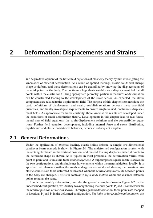
2Deformation:Displacements and Strains We begin development of the basicfield equations of elasticity theory byfirst investigating thekinematics of material deformation.As a result of applied loadings,elastic solids will changeshape or deform,and these deformations can be quantified by knowing the displacements ofmaterial points in the body.The continuum hypothesis establishes a displacementfield at allpoints within the elastic ing appropriate geometry,particular measures of deformationcan be constructed leading to the development of the strain tensor.As expected,the straincomponents are related to the displacementfield.The purpose of this chapter is to introduce thebasic definitions of displacement and strain,establish relations between these twofieldquantities,andfinally investigate requirements to ensure single-valued,continuous displace-mentfields.As appropriate for linear elasticity,these kinematical results are developed underthe conditions of small deformation theory.Developments in this chapter lead to two funda-mental sets offield equations:the strain-displacement relations and the compatibility equa-tions.Furtherfield equation development,including internal force and stress distribution,equilibrium and elastic constitutive behavior,occurs in subsequent chapters.2.1General DeformationsUnder the application of external loading,elastic solids deform.A simple two-dimensionalcantilever beam example is shown in Figure2-1.The undeformed configuration is taken withthe rectangular beam in the vertical position,and the end loading displaces material points tothe deformed shape as shown.As is typical in most problems,the deformation varies frompoint to point and is thus said to be nonhomogenous.A superimposed square mesh is shown inthe two configurations,and this indicates how elements within the material deform locally.It isapparent that elements within the mesh undergo extensional and shearing deformation.Anelastic solid is said to be deformed or strained when the relative displacements between pointsin the body are changed.This is in contrast to rigid-body motion where the distance betweenpoints remains the same.In order to quantify deformation,consider the general example shown in Figure2-2.In the undeformed configuration,we identify two neighboring material points P o and P connected withthe relative position vector r as shown.Through a general deformation,these points are mappedand P0in the deformed configuration.Forfinite or large deformation theory,the to locations P0o27undeformed and deformed configurations can be significantly different,and a distinction between these two configurations must be maintained leading to Lagrangian and Eulerian descriptions;see,for example,Malvern(1969)or Chandrasekharaiah and Debnath(1994). However,since we are developing linear elasticity,which uses only small deformation theory, the distinction between undeformed and deformed configurations can be dropped.Using Cartesian coordinates,define the displacement vectors of points P o and P to be u o and u,respectively.Since P and P o are neighboring points,we can use a Taylor series expansion around point P o to express the components of u asu¼u oþ@u@xr xþ@u@yr yþ@u@zr zv¼v oþ@v@xr xþ@v@yr yþ@v@zr zw¼w oþ@w@xr xþ@w@yr yþ@w@zr z(2:1:1)FIGURE2-1Two-dimensional deformation example.(Undeformed)(Deformed) FIGURE2-2General deformation between two neighboring points.28FOUNDATIONS AND ELEMENTARY APPLICATIONSNote that the higher-order terms of the expansion have been dropped since the components of r are small.The change in the relative position vector r can be written asD r¼r0Àr¼uÀu o(2:1:2) and using(2.1.1)givesD r x¼@u@xr xþ@u@yr yþ@u@zr zD r y¼@v@xr xþ@v@yr yþ@v@zr zD r z¼@w@xr xþ@w@yr yþ@w@zr z(2:1:3)or in index notationD r i¼u i,j r j(2:1:4) The tensor u i,j is called the displacement gradient tensor,and may be written out asu i,j¼@u@x@u@y@u@z@v@x@v@y@v@z@w@x@w@y@w@z2666666437777775(2:1:5)From relation(1.2.10),this tensor can be decomposed into symmetric and antisymmetric parts asu i,j¼e ijþ!ij(2:1:6) wheree ij¼12(u i,jþu j,i)!ij¼12(u i,jÀu j,i)(2:1:7)The tensor e ij is called the strain tensor,while!ij is referred to as the rotation tensor.Relations (2.1.4)and(2.1.6)thus imply that for small deformation theory,the change in the relative position vector between neighboring points can be expressed in terms of a sum of strain and rotation bining relations(2.1.2),(2.1.4),and(2.1.6),and choosing r i¼dx i, we can also write the general result in the formu i¼u o iþe ij dx jþ!ij dx j(2:1:8) Because we are considering a general displacementfield,these results include both strain deformation and rigid-body motion.Recall from Exercise1-14that a dual vector!i canDeformation:Displacements and Strains29be associated with the rotation tensor such that !i ¼À1=2e ijk !jk .Using this definition,it is found that!1¼!32¼12@u 3@x 2À@u 2@x 3 !2¼!13¼12@u 1@x 3À@u 3@x 1 !3¼!21¼12@u 2@x 1À@u 1@x 2 (2:1:9)which can be expressed collectively in vector format as v ¼(1=2)(r Âu ).As is shown in the next section,these components represent rigid-body rotation of material elements about the coordinate axes.These general results indicate that the strain deformation is related to the strain tensor e ij ,which in turn is a related to the displacement gradients.We next pursue a more geometric approach and determine specific connections between the strain tensor components and geometric deformation of material elements.2.2Geometric Construction of Small Deformation TheoryAlthough the previous section developed general relations for small deformation theory,we now wish to establish a more geometrical interpretation of these results.Typically,elasticity variables and equations are field quantities defined at each point in the material continuum.However,particular field equations are often developed by first investigating the behavior of infinitesimal elements (with coordinate boundaries),and then a limiting process is invoked that allows the element to shrink to a point.Thus,consider the common deformational behavior of a rectangular element as shown in Figure 2-3.The usual types of motion include rigid-body rotation and extensional and shearing deformations as illustrated.Rigid-body motion does not contribute to the strain field,and thus also does not affect the stresses.We therefore focus our study primarily on the extensional and shearing deformation.Figure 2-4illustrates the two-dimensional deformation of a rectangular element with original dimensions dx by dy .After deformation,the element takes a rhombus form as shown in the dotted outline.The displacements of various corner reference points areindicated(Rigid Body Rotation)(Undeformed Element)(Horizontal Extension)(Vertical Extension)(Shearing Deformation)FIGURE 2-3Typical deformations of a rectangular element.30FOUNDATIONS AND ELEMENTARY APPLICATIONSin the figure.Reference point A is taken at location (x,y ),and the displacement components of this point are thus u (x,y )and v (x,y ).The corresponding displacements of point B are u (x þdx ,y )and v (x þdx ,y ),and the displacements of the other corner points are defined in an analogous manner.According to small deformation theory,u (x þdx ,y )%u (x ,y )þ(@u =@x )dx ,with similar expansions for all other terms.The normal or extensional strain component in a direction n is defined as the change in length per unit length of fibers oriented in the n -direction.Normal strain is positive if fibers increase in length and negative if the fiber is shortened.In Figure 2-4,the normal strain in the x direction can thus be defined bye x ¼A 0B 0ÀAB From the geometry in Figure 2-4,A 0B 0¼ffiffiffiffiffiffiffiffiffiffiffiffiffiffiffiffiffiffiffiffiffiffiffiffiffiffiffiffiffiffiffiffiffiffiffiffiffiffiffiffiffiffiffiffiffiffiffiffiffiffiffiffiffidx þ@u @x dx 2þ@v @x dx 2s ¼ffiffiffiffiffiffiffiffiffiffiffiffiffiffiffiffiffiffiffiffiffiffiffiffiffiffiffiffiffiffiffiffiffiffiffiffiffiffiffiffiffiffiffiffiffiffiffiffiffiffiffiffiffiffiffiffiffiffiffi1þ2@u @x þ@u @x 2þ@v @x 2dx s %1þ@u @xdx where,consistent with small deformation theory,we have dropped the higher-order ing these results and the fact that AB ¼dx ,the normal strain in the x -direction reduces toe x ¼@u@x (2:2:1)In similar fashion,the normal strain in the y -direction becomese y ¼@v@y (2:2:2)A second type of strain is shearing deformation,which involves angles changes (see Figure 2-3).Shear strain is defined as the change in angle between two originally orthogonalx FIGURE 2-4Two-dimensional geometric strain deformation.Deformation:Displacements and Strains 31directions in the continuum material.This definition is actually referred to as the engineering shear strain.Theory of elasticity applications generally use a tensor formalism that requires a shear strain definition corresponding to one-half the angle change between orthogonal axes; see previous relation(2:1:7)1.Measured in radians,shear strain is positive if the right angle between the positive directions of the two axes decreases.Thus,the sign of the shear strain depends on the coordinate system.In Figure2-4,the engineering shear strain with respect to the x-and y-directions can be defined asg xy¼p2ÀffC0A0B0¼aþbFor small deformations,a%tan a and b%tan b,and the shear strain can then be expressed asg xy¼@v@xdxdxþ@u@xdxþ@u@ydydyþ@v@ydy¼@u@yþ@v@x(2:2:3)where we have again neglected higher-order terms in the displacement gradients.Note that each derivative term is positive if lines AB and AC rotate inward as shown in thefigure.By simple interchange of x and y and u and v,it is apparent that g xy¼g yx.By considering similar behaviors in the y-z and x-z planes,these results can be easily extended to the general three-dimensional case,giving the results:e x¼@u@x,e y¼@v@y,e z¼@w@zg xy¼@u@yþ@v@x,g yz¼@v@zþ@w@y,g zx¼@w@xþ@u@z(2:2:4)Thus,we define three normal and three shearing strain components leading to a total of six independent components that completely describe small deformation theory.This set of equations is normally referred to as the strain-displacement relations.However,these results are written in terms of the engineering strain components,and tensorial elasticity theory prefers to use the strain tensor e ij defined by(2:1:7)1.This represents only a minor change because the normal strains are identical and shearing strains differ by a factor of one-half;for example,e11¼e x¼e x and e12¼e xy¼1=2g xy,and so forth.Therefore,using the strain tensor e ij,the strain-displacement relations can be expressed in component form ase x¼@u@x,e y¼@v@y,e z¼@w@ze xy¼1@uþ@v,e yz¼1@vþ@w,e zx¼1@wþ@u(2:2:5)Using the more compact tensor notation,these relations are written ase ij¼12(u i,jþu j,i)(2:2:6)32FOUNDATIONS AND ELEMENTARY APPLICATIONSwhile in direct vector/matrix notation as the form reads:e¼12r uþ(r u)TÂÃ(2:2:7)where e is the strain matrix and r u is the displacement gradient matrix and(r u)T is its transpose.The strain is a symmetric second-order tensor(e ij¼e ji)and is commonly written in matrix format:e¼[e]¼e x e xy e xze xy e y e yze xz e yz e z2435(2:2:8)Before we conclude this geometric presentation,consider the rigid-body rotation of our two-dimensional element in the x-y plane,as shown in Figure2-5.If the element is rotated through a small rigid-body angular displacement about the z-axis,using the bottom element edge,the rotation angle is determined as@v=@x,while using the left edge,the angle is given byÀ@u=@y. These two expressions are of course the same;that is,@v=@x¼À@u=@y and note that this would imply e xy¼0.The rotation can then be expressed as!z¼[(@v=@x)À(@u=@y)]=2, which matches with the expression given earlier in(2:1:9)3.The other components of rotation follow in an analogous manner.Relations for the constant rotation!z can be integrated to give the result:u*¼u oÀ!z yv*¼v oþ!z x(2:2:9)where u o and v o are arbitrary constant translations in the x-and y-directions.This result then specifies the general form of the displacementfield for two-dimensional rigid-body motion.We can easily verify that the displacementfield given by(2.2.9)yields zero strain.xFIGURE2-5Two-dimensional rigid-body rotation.Deformation:Displacements and Strains33For the three-dimensional case,the most general form of rigid-body displacement can beexpressed asu*¼u oÀ!z yþ!y zv*¼v oÀ!x zþ!z xw*¼w oÀ!y xþ!x y(2:2:10)As shown later,integrating the strain-displacement relations to determine the displacementfield produces arbitrary constants and functions of integration,which are equivalent to rigid-body motion terms of the form given by(2.2.9)or(2.2.10).Thus,it is important to recognizesuch terms because we normally want to drop them from the analysis since they do notcontribute to the strain or stressfields.2.3Strain TransformationBecause the strains are components of a second-order tensor,the transformation theorydiscussed in Section1.5can be applied.Transformation relation(1:5:1)3is applicable forsecond-order tensors,and applying this to the strain givese0ij¼Q ip Q jq e pq(2:3:1)where the rotation matrix Q ij¼cos(x0i,x j).Thus,given the strain in one coordinate system,we can determine the new components in any other rotated system.For the general three-dimensional case,define the rotation matrix asQ ij¼l1m1n1l2m2n2l3m3n32435(2:3:2)Using this notational scheme,the specific transformation relations from equation(2.3.1)becomee0x¼e x l21þe y m21þe z n21þ2(e xy l1m1þe yz m1n1þe zx n1l1)e0y¼e x l22þe y m22þe z n22þ2(e xy l2m2þe yz m2n2þe zx n2l2)e0z¼e x l23þe y m23þe z n23þ2(e xy l3m3þe yz m3n3þe zx n3l3)e0xy¼e x l1l2þe y m1m2þe z n1n2þe xy(l1m2þm1l2)þe yz(m1n2þn1m2)þe zx(n1l2þl1n2)e0yz¼e x l2l3þe y m2m3þe z n2n3þe xy(l2m3þm2l3)þe yz(m2n3þn2m3)þe zx(n2l3þl2n3)e0zx¼e x l3l1þe y m3m1þe z n3n1þe xy(l3m1þm3l1)þe yz(m3n1þn3m1)þe zx(n3l1þl3n1)(2:3:3)For the two-dimensional case shown in Figure2-6,the transformation matrix can be ex-pressed asQ ij¼cos y sin y0Àsin y cos y00012435(2:3:4)34FOUNDATIONS AND ELEMENTARY APPLICATIONSUnder this transformation,the in-plane strain components transform according toe 0x ¼e x cos 2y þe y sin 2y þ2e xy sin y cos ye 0y ¼e x sin 2y þe y cos 2y À2e xy sin y cos ye 0xy ¼Àe x sin y cos y þe y sin y cos y þe xy (cos 2y Àsin 2y )(2:3:5)which is commonly rewritten in terms of the double angle:e 0x ¼e x þe y 2þe x Àe y 2cos 2y þe xy sin 2y e 0y ¼e x þe y Àe x Àe y cos 2y Àe xy sin 2y e 0xy ¼e y Àe x 2sin 2y þe xy cos 2y (2:3:6)Transformation relations (2.3.6)can be directly applied to establish transformations between Cartesian and polar coordinate systems (see Exercise 2-6).Additional applications of these results can be found when dealing with experimental strain gage measurement systems.For example,standard experimental methods using a rosette strain gage allow the determination of extensional strains in three different directions on the surface of a ing this type of data,relation (2:3:6)1can be repeatedly used to establish three independent equations that can be solved for the state of strain (e x ,e y ,e xy )at the surface point under study (see Exercise 2-7).Both two-and three-dimensional transformation equations can be easily incorporated in MATLAB to provide numerical solutions to problems of interest.Such examples are given in Exercises 2-8and 2-9.2.4Principal StrainsFrom the previous discussion in Section 1.6,it follows that because the strain is a symmetric second-order tensor,we can identify and determine its principal axes and values.According to this theory,for any given strain tensor we can establish the principal value problem and solvey ′FIGURE 2-6Two-dimensional rotational transformation.Deformation:Displacements and Strains 35the characteristic equation to explicitly determine the principal values and directions.The general characteristic equation for the strain tensor can be written asdet[e ijÀe d ij]¼Àe3þW1e2ÀW2eþW3¼0(2:4:1) where e is the principal strain and the fundamental invariants of the strain tensor can be expressed in terms of the three principal strains e1,e2,e3asW1¼e1þe2þe3W2¼e1e2þe2e3þe3e1W3¼e1e2e3(2:4:2)Thefirst invariant W1¼W is normally called the cubical dilatation,because it is related to the change in volume of material elements(see Exercise2-11).The strain matrix in the principal coordinate system takes the special diagonal forme ij¼e1000e2000e32435(2:4:3)Notice that for this principal coordinate system,the deformation does not produce anyshearing and thus is only extensional.Therefore,a rectangular element oriented alongprincipal axes of strain will retain its orthogonal shape and undergo only extensional deform-ation of its sides.2.5Spherical and Deviatoric StrainsIn particular applications it is convenient to decompose the strain tensor into two parts calledspherical and deviatoric strain tensors.The spherical strain is defined by~e ij¼13e kk d ij¼13Wd ij(2:5:1)while the deviatoric strain is specified as^e ij¼e ijÀ13e kk d ij(2:5:2)Note that the total strain is then simply the sume ij¼~e ijþ^e ij(2:5:3)The spherical strain represents only volumetric deformation and is an isotropic tensor,being the same in all coordinate systems(as per the discussion in Section1.5).The deviatoricstrain tensor then accounts for changes in shape of material elements.It can be shownthat the principal directions of the deviatoric strain are the same as those of the straintensor.36FOUNDATIONS AND ELEMENTARY APPLICATIONS2.6Strain CompatibilityWe now investigate in more detail the nature of the strain-displacement relations (2.2.5),and this will lead to the development of some additional relations necessary to ensure continuous,single-valued displacement field solutions.Relations (2.2.5),or the index notation form (2.2.6),represent six equations for the six strain components in terms of three displacements.If we specify continuous,single-valued displacements u,v,w,then through differentiation the resulting strain field will be equally well behaved.However,the converse is not necessarily true;that is,given the six strain components,integration of the strain-displacement relations (2.2.5)does not necessarily produce continuous,single-valued displacements.This should not be totally surprising since we are trying to solve six equations for only three unknown displacement components.In order to ensure continuous,single-valued displacements,the strains must satisfy additional relations called integrability or compatibility equations .Before we proceed with the mathematics to develop these equations,it is instructive to consider a geometric interpretation of this concept.A two-dimensional example is shown in Figure 2-7whereby an elastic solid is first divided into a series of elements in case (a).For simple visualization,consider only four such elements.In the undeformed configuration shown in case (b),these elements of course fit together perfectly.Next,let us arbitrarily specify the strain of each of the four elements and attempt to reconstruct the solid.For case (c),the elements have been carefully strained,taking into consideration neighboring elements so that the system fits together thus yielding continuous,single-valued displacements.However,for(b) Undeformed Configuration(c) Deformed ConfigurationContinuous Displacements (a) Discretized Elastic Solid (d) Deformed Configuration Discontinuous DisplacementsFIGURE 2-7Physical interpretation of strain compatibility.case(d),the elements have been individually deformed without any concern for neighboring deformations.It is observed for this case that the system will notfit together without voids and gaps,and this situation produces a discontinuous displacementfield.So,we again conclude that the strain components must be somehow related to yield continuous,single-valued displacements.We now pursue these particular relations.The process to develop these equations is based on eliminating the displacements from the strain-displacement relations.Working in index notation,we start by differentiating(2.2.6) twice with respect to x k and x l:e ij,kl¼12(u i,jklþu j,ikl)Through simple interchange of subscripts,we can generate the following additional relations:e kl,ij¼12(u k,lijþu l,kij)e jl,ik¼12(u j,likþu l,jik)e ik,jl¼12(u i,kjlþu k,ijl)Working under the assumption of continuous displacements,we can interchange the order of differentiation on u,and the displacements can be eliminated from the preceding set to gete ij,klþe kl,ijÀe ik,jlÀe jl,ik¼0(2:6:1) These are called the Saint Venant compatibility equations.Although the system would lead to 81individual equations,most are either simple identities or repetitions,and only6are meaningful.These six relations may be determined by letting k¼l,and in scalar notation, they become@2e x @y2þ@2e y@x2¼2@2e xy@x@y@2e y @z2þ@2e z@y2¼2@2e yz@y@z@2e z @x2þ@2e x@z2¼2@2e zx@z@x@2e x @y@z ¼@@xÀ@e yz@xþ@e zx@yþ@e xy@z@2e y @z@x ¼@@yÀ@e zx@yþ@e xy@zþ@e yz@x@2e z @x@y ¼@@zÀ@e xy@zþ@e yz@xþ@e zx@y(2:6:2)It can be shown that these six equations are equivalent to three independent fourth-order relations(see Exercise2-14).However,it is usually more convenient to use the six second-order equations given by(2.6.2).In the development of the compatibility relations,we assumed that the displacements were continuous,and thus the resulting equations (2.6.2)are actually only a necessary condition.In order to show that they are also sufficient,consider two arbitrary points P and P o in an elastic solid,as shown in Figure 2-8.Without loss in generality,the origin may be placed at point P o .The displacements of points P and P o are denoted by u P i and u o i ,and the displacement ofpoint P can be expressed asu P i ¼u o i þðC du i ¼u o i þðC @u i @x j dx j (2:6:3)where C is any continuous curve connecting points P o and P .Using relation (2.1.6)for the displacement gradient,(2.6.3)becomesu P i ¼u o i þðC (e ij þ!ij )dx j (2:6:4)Integrating the last term by parts givesðC !ij dx j ¼!P ij x P j ÀðC x j !ij ,k dx k (2:6:5)where !P ij is the rotation tensor at point P .Using relation (2:1:7)2,!ij ,k ¼12(u i ,jk Àu j ,ik )¼12(u i ,jk Àu j ,ik )þ12(u k ,ji Àu k ,ji )¼12@@x j (u i ,k þu k ,i )À12@@x i(u j ,k þu k ,j )¼e ik ,j Àe jk ,i (2:6:6)Substituting results (2.6.5)and (2.6.6)into (2.6.4)yieldsu P i¼u o i þ!P ij x P j þðC U ik dx k (2:6:7)where U ik ¼e ik Àx j (e ik ,j Àe jk ,i ).P oFIGURE 2-8Continuity of displacements.Now if the displacements are to be continuous,single-valued functions,the line integral appearing in(2.6.7)must be the same for any curve C;that is,the integral must be independent of the path of integration.This implies that the integrand must be an exact differential,so that the value of the integral depends only on the end points.Invoking Stokes theorem,we can show that if the region is simply connected(definition of the term simply connected is postponed for the moment),a necessary and sufficient condition for the integral to be path independent is for U ik,l¼U il,ing this result yieldse ik,lÀd jl(e ik,jÀe jk,i)Àx j(e ik,jlÀe jk,il)¼e il,kÀd jk(e il,jÀe jl,i)Àx j(e il,jkÀe jl,ik) which reduces tox j(e ik,jlÀe jk,ilÀe il,jkþe jl,ik)¼0Because this equation must be true for all values of x j,the terms in parentheses must vanish, and after some index renaming this gives the identical result previously stated by the compati-bility relations(2.6.1):e ij,klþe kl,ijÀe ik,jlÀe jl,ik¼0Thus,relations(2.6.1)or(2.6.2)are the necessary and sufficient conditions for continuous, single-valued displacements in simply connected regions.Now let us get back to the term simply connected.This concept is related to the topology or geometry of the region under study.There are several places in elasticity theory where the connectivity of the region fundamentally affects the formulation and solution method. The term simply connected refers to regions of space for which all simple closed curves drawn in the region can be continuously shrunk to a point without going outside the region. Domains not having this property are called multiply connected.Several examples of such regions are illustrated in Figure2-9.A general simply connected two-dimensional region is shown in case(a),and clearly this case allows any contour within the region to be shrunk to a point without going out of the domain.However,if we create a hole in the region as shown in case(b),a closed contour surrounding the hole cannot be shrunk to a point without going into the hole and thus outside of the region.Thus,for two-dimensional regions,the presence of one or more holes makes the region multiply connected.Note that by introducing a cut between the outer and inner boundaries in case(b),a new region is created that is now simply connected. Thus,multiply connected regions can be made simply connected by introducing one or more cuts between appropriate boundaries.Case(c)illustrates a simply connected three-dimensional example of a solid circular cylinder.If a spherical cavity is placed inside this cylinder as shown in case(d),the region is still simply connected because any closed contour can still be shrunk to a point by sliding around the interior cavity.However,if the cylinder has a through hole as shown in case(e),then an interior contour encircling the axial through hole cannot be reduced to a point without going into the hole and outside the body.Thus,case(e)is an example of the multiply connected three-dimensional region.It was found that the compatibility equations are necessary and sufficient conditions for continuous,single-valued displacements only for simply connected regions.However, for multiply connected domains,relations(2.6.1)or(2.6.2)provide only necessary but。
弹性力学讲义绪论p

§1-2 弹性力学的发展
第1章 绪论1-2
线性问题发展期(约于1854 一1907 )
A.Castigliano( 意)(卡斯蒂利亚诺 )—1873-1879 , 建立了最小余能原理 D.C.L.Rayleigh;W.Ritz (瑞利一里茨)—1877-1908, 提出了Rayleigh-Ritz 法 B.G.Galerkin (俄)(伽辽金法)—1915, 迦辽金近似 计算法
合的构架等。
§1-1 弹性力学的内容
弹性力学与材料力学等学科的比较
第1章 绪论1-1
构件承载能力分析是固体力学的基本任务
不同的学科分支,研究对象和方法是不同的
从研究对象看 从研究的方法上看
§1-1 弹性力学的内容
弹性力学与材料力学等学科的比较
第1章 绪论1-1
? 研究对象——弹性体—近似 ?研究内容和基本任务—基本相同 ?研究方法—却有比较大的差别
《弹性力学》教学大纲
教材要求
建议教材: 陈国荣.弹性力学.
南京:河海大学出版社,2002
参考书:S.P.Timoshenko. Theory of Elasticity (Third Edition)
内容与初步安排: (共48学时)
第1章 绪论(3学时) 第2章 平面应力与平面应变(5学时) 第3章 平面问题的直角坐标解答(4学时) 第4章 平面问题的极坐标解答 (6学时) 第5章 三维问题的基本理论 (8学时) 第6章 三维问题的基本解法与弹性力学的一般原理(4学时
§1-2 弹性力学的发展
第1章 绪论1-2
非线性问题发展期(1907一)
1907年,卡门首先提出了薄板大挠度问题(大位移)
1937-1939 ,F.D.Murnaghan;M.A.Biot 提出大应 变问题
弹性力学课件全本
© 2006.Wei Yuan. All rights reserved.
2. 应力:单位截面面积的内力.
内力:发生在物体内部的力,即物体 本身不同部分之间相互作用的力。
lim
ΔV 0
z
Ⅱ
F A p P
Ⅰ
F p A
o x
y
p: 极限矢量,即物体在截面mn上的、在P点的应力。 方向就是F的极限方向。 应力分量:, 量纲:N/m2=kg∙m/s2∙m2=kg/m∙s2 即:L-1MT-2
(Theory of Elasticity),研究弹性体由于受外力、边界
约束或温度改变等原因而发生的应力、形变和位移。 研究对象:弹性体 研究目标:变形等效应,即应力、形变和位移。
2. 对弹性力学、材料力学和结构力学作比较
弹性力学的任务和材料力学, 结构力学的任务一样, 是分析各种结构物或其构件在弹性阶段的应力和位 移, 校核它们是否具有所需的强度和刚度, 并寻求或 改进它们的计算方法.
x
zx
A
y
可以证明,已知x, y, z, yz, zx, xy, 就可求得经过 该点任一线段上的线应变 .也可以求得经过该点任 意两个线段之间的角度的改变。因此,此六个形变 分量可以完全确定该点的形变状态。
© 2006.Wei Yuan. All rights reserved.
(2)研究方法: 弹性力学与材料力学有相似,又有一 定区别。
© 2006.Wei Yuan. All rights reserved.
弹性力学:在弹性体区域内必须严格考虑静力学、 几何学和物理学三方面条件,在边界上严格考虑受 力条件或约束条件,由此建立微分方程和边界条件 进行求解,得出精确解答。 材料力学:虽然也考虑这几个方面的的条件,但不是 十分严格。
弹性力学双语讲义(chapter1)
extbook: Applied Elasticity 徐芝纶 中文教材: 中文教材: 弹性力学简明教程 徐芝纶
Chapter 1. Introduction 第一章 绪论
•A prismatical tension member with a small hole •It is assumed in mechanics of materials that the tensile stresses are uniformly distributed across the net section of the member. •The analysis in elasticity shows that the stresses are by no means uniform, but are concentrated near the hole.
Three branches of solid mechanics 固体力学的三个分枝 固体力学的三个分枝
• Mechanics of materials 材料力学, 材料力学, Structural Mechanics 结构力学 Elasticity 弹性力学
•
•
What does the Elasticity deal with? It deals with the stresses, deformations and displacements in elastic solids produced by external forces or changes in temperature. 研究弹性体由于外力和温度改变而引起的应力, 由于外力和温度改变而引起的应力 研究弹性体由于外力和温度改变而引起的应力, 形变和位移。 形变和位移。 It analyzes the stresses, deformations and displacements of structural elements within the elastic range and thereby to check the sufficiency of their strength, stiffness and stability. 分析结构的应力,形变和位移, 分析结构的应力,形变和位移,检查是否满足强 刚度和稳定性条件。 度,刚度和稳定性条件。
弹性力学2
弹性力学简明教程第一章绪论1.弹性力学:又称为弹性理论,是固体力学的一个分支,其中研究弹性体由于受到外力作用、边界约束或温度改变等原因而发生的应力、形变和位移。
2. 作用于物体的外力可以分为两种:一种是分布在物体表面的作用力,例如一个物体对另一物体作用的压力,象水压力等,称做面力;另一种是分布在物体体积内的力,象重力、磁力或运动物体的惯性力等,称为体力。
3.内力:物体本身不同部分之间相互作用的力。
4.弹性力学的基本假定:1假定物体处处连续;2假定物体是完全弹性的;3假定物体是均匀的;4假定物体是各向同性的;5假定位移和形变很小。
(满足前四个为理想弹性体)第二章平面问题的基本理论一、弹性力学空间问题共有应力、应变和位移15个未知函数,且均为。
二、弹性力学平面问题共有应力、应变和位移8个未知函数,且均为。
三、平面应力问题:(1)等厚度的薄板;(2)体力作用于体内,平行于板的中面,沿板厚不变;(3)面力作用于板边,平行于板的中面,沿板厚不变;(4)约束作用于板边,平行于板的中面,沿板厚不变。
四、平面应变问题:(1)很长的常截面柱体;(2)体力作用于体内,平行于横截面,沿柱体长度方向不变;(3)面力作用于柱面,平行于横截面,沿柱体长度方向不变;(4)约束作用于柱面,平行于横截面,沿柱体长度方向不变。
五、挡土墙和很长的管道、隧洞问题,是很接近于平面应变问题。
六、平衡微分方程:七、边界条件--表示在边界上位移与约束,或应力与面力之间的关系。
(分为位移边界条件、应力边界条件、混合边界条件)八、圣维南原理:如果把物体的一小部分边界上的面力,变换为分布不同但静力等效的面力(主矢量相同,对同一点的主矩也相同),那么,近处的应力分量将著的改变,但远处所受的影响可以不计。
九、静力等效─指两者主矢量相同,对同一点主矩也相同;十、圣维南原理表明,在小边界上进行面力的静力等效变换后,只影响近处(局部区域)的应力,对绝大部分弹性体区域的应力没有明显影响。
弹性力学基本讲义
三个平面内的剪应变:
x , y , z xy , yz , zx
z C
z
A
O
应变的正负: 线应变: 伸长时为正,缩短时为负;
剪应变: 以直角变小时为正,变大时为负; x
x P
y
B y
(2) 一点应变状态
—— 代表一点 P 的邻域内线段与线段间夹角的改变
x yx zx
(3)数学理论基础 材力、结力 —— 常微分方程(4阶,一个变量)。 弹力 —— 偏微分方程(高阶,二、三个变量)。
数值解法:能量法(变分法)、差分 法、有限单元法等。 3. 与其他力学课程的关系
数学弹性力学;
弹性力学
应用弹性力学。
弹性力学是塑性力学、断裂力学、岩石力学、 土力学、振动理论、有限单元法等课程的基础。
三、线性理论的发展时期(约1854-1907年) *应用建立的线弹性理论,解决大量工程实际问题,并推动 了数学分析工作的进展。 代表性的事件:(1) 圣维南(1854-1856年)提出圣维南原理; (2) 艾里(1862年)提出了求解平面问题的应力函数;(3) 赫兹(1882 年)求解了接触问题;基尔霍夫(1850年及以后)解决了平板的平 衡和振动问题。弹性力学在该时期得到了飞跃发展。 四、弹性力学更深入的发展时期(约1907年至今) *非线性弹性力学迅速发展起来。 代表性的事件:(1) 卡门(1907年)提出薄板的大挠度问题; (2) 卡门和钱学森提出了薄壳的非线性稳定问题;(3) 其他学者 还提出了大应变问题,非线性材料问题如塑性力学等。
1, 1
作用: 建立方程时,可略去高阶微量;
可用变形前的尺寸代替变形后的尺寸。 使求解的方程线性化。
清华大学研究生弹塑性力学讲义 5弹塑性_弹性力学的基本方程与解法
弹塑性力学第四章 弹性力学的基本方程与解法一、线性弹性理论适定问题的基本方程和边界条件对于在空间占有体积域V 的线弹性体在外加恒定载荷和固定几何约束条件下引起的小变形问题,若以, ,u εσ作为求解变量,则可以建立如下偏微分方程边值问题: 几何方程()1,,2ij i j j i u u ε=+ ()12∇+∇u u ε= (1a)广义胡克定律 ij ijkl kl E σε= :E σ=ε(1b)平衡方程 ,0ij j i f σ+= ∇⋅+=f 0σ V∀∈x (1c)以上方程均要求在域内各点均满足。
边界条件 u u i i = ∀∈x S ui (2a)n t j ji i σ= ∀∈x S ti(2b)对于适定问题,即不仅要求保证解存在唯一,而且有较好的稳定性。
当载荷或边界条件给定值有微小摄动时,应能保证问题解的变化也是微小的。
对于边界条件的提法就有严格的要求。
即要求:S S S S S ui ti ui ti U I ==∅(2c)对于各向同性材料,其广义胡克定律可具体写成 σλεδεij kk ij ij G =+2 ()tr 2G λ+I σ=εε (3a)()11ij ij kk ij E ενσνσδ⎡⎤=+−⎣⎦ ()()1tr Eνν=⎡⎤⎣⎦I ε1+σ−σ (3b)以上就域内方程来说,一共是对于u ,,σ ε的15个独立分量u i ij ij ,, σε的15个方程。
对于边界条件来说,三维问题每点有三个边界条件,而且是在三个正交方向上每个方向有一个边界条件,这个边界条件或者给定位移、或者给定面力。
这三个正交第四章 弹性力学的基本方程与解法方向可以是整体笛卡儿坐标系的三个方向,也可以是边界自然坐标系的三个方向(即法向和两个切向)。
从更一般来说,除去给定位移或面力外,还有另一种线性的边界条件t K u c i ij j i +=(4)这是一种弹性约束条件。
用这个条件可以取代给定位移或给定面力的条件。
弹性力学讲课文档

因此,即应力与应变关系可用胡克定律表示 (物理线性)。
31
第三十一页,共39页。
(3)均匀性--假定物体由同种材料组成。
因此, E、μ等与位置 无关。 (4)各向同性--假定物体各向同性。
因此, E、μ等与方向无关。
由(3),(4)知E、μ等为常数 符合(1)-(4)假定的称为理想弹性体。
21
第二十一页,共39页。
z
oy x
yz
σy
yx
图1-6
(2)符号规定:
图示单元体面的法线为y,称为y
面,应力分量垂直于单元体面的应 力称为正应力。
正应力记为σy,沿y轴的正向 为正,其下标表示所沿坐标轴的方向
。
平行于单元体面的应力称为切
应下力标,y表用示所在、yx的平面表yz,示第,二其下第标一x
、z分别表示沿坐标轴的方向。如
图1-6所示的 、 yx。 yz
22
第二十二页,共39页。
其它x、z正面上的应力
分量的表示如图1-7所示。
凡正面上的应力沿坐
标正向为正,逆坐标正向
z
为负。
图1-7
oy
x
23
第二十三页,共39页。
z
oy x
图1-8
图1-8所示单元体
面的法线为y的负向,正
应力记为
,沿y轴负向
37
第三十七页,共39页。
《绪论》习题课
[练习2]弹性力学中基本假设是什么?
答:为了简化计算,弹性力学中采用如下基本假设: (1)连续性假设,(2)完全弹性假设,(3)均匀性假 设,(4)各向同性假设,(5)小变形假设。
38
第三十八页,共39页。
弹性力学第一章
•The analysis in elasticity shows that the stresses are by no means uniform, but are concentrated near the hole.
•No assumption, that a plane section of the beam remains plane after bending, is made in Elasticity.
弹性力学 第一章
19
•A prismatical tension member with a small hole
弹性力学 第一章
7
Comparison among the three courses in solid mechanics
固体力学三门学科的比较
• Three branches have the same purpose and do differ from one another both in objects studied and the methods of analysis used.
Elasticity: 弹性力学
1. plates and shells 板,壳 2.blocks: 块体 e.g. dams,foundations 坝,基础
3.analyze bar element precisely 对杆件作精确分析
弹性力学 第一章
弹性力学讲义
弹性力学01绪论1.1弹性力学的内容1.2弹性力学的几个基本概念 1.3弹性力学中的基本假定。
1.1、弹性力学的内容弹性力学:研究弹性体由于受外力、边界约束或温度等原因而发生的应力、变形和位移。
研究弹性体的力学:有材料力学、结构力学、弹性力学。
它们的研究对象分别如下: ①材料力学:研究杆件(如梁、柱和轴)的拉压、弯曲、剪切、扭转和组合变形等问题。
②结构力学:在材料力学基础上研究杆系结构(如桁架、钢架等)③弹性力学:研究各种形状的弹性体,如杆件、平面体、空间体、板壳、薄壁结构等问题。
在研究方法上,弹性力学和材料力学也有区别:弹力研究方法:在区域V 内严格考虑静力学、几何学和物理学三方面条件,建立三套方程;在边界s 上考虑受力或约束条件,并在边界条件下求解上述方程,得出较精确的解答。
材力也考虑这几方面的条件,但不是十分严格的:常常引用近似的计算假设(如平面截面假设)来简化问题,并在许多方面进行了近似的处理。
因此材料力学建立的是近似理论,得出的是近似的解答。
从其精度来看,材料力学解法只能适用于杆件。
例如:材料力学:研究直梁在横向载荷作用下的平面弯曲,引用了平面假设,结果:横截面上的正应力按直线分布。
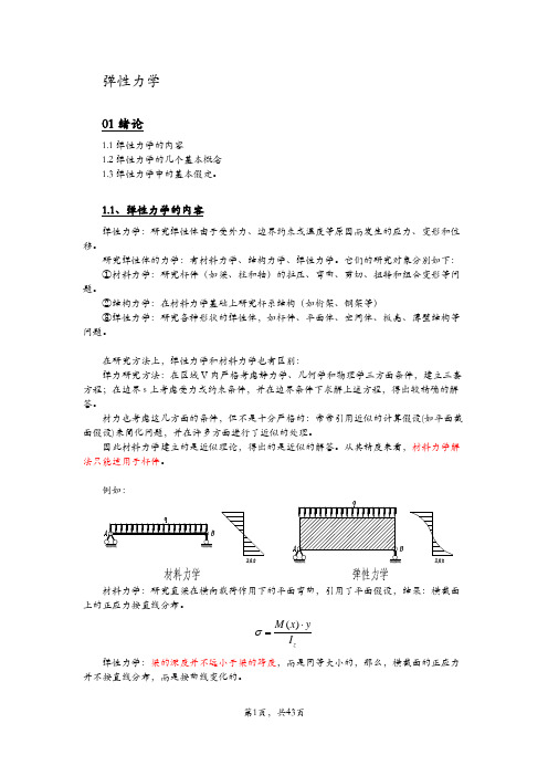
()zM x yI σ⋅=弹性力学:梁的深度并不远小于梁的跨度,而是同等大小的,那么,横截面的正应力并不按直线分布,而是按曲线变化的。
22()345z M x y y y q I h h σ⎛⎫⋅=+- ⎪⎝⎭这时,材料力学中给出的最大正应力将具有很大的误差。
弹性力学在力学学科和工程学科中,具有重要的地位:弹性力学是其他固体力学分支学科的基础。
弹性力学是工程结构分析的重要手段。
尤其对于安全性和经济性要求很高的近代大型工程结构,须用弹力方法进行分析。
工科学生学习弹力的目的:1)理解和掌握弹力的基本理论; 2)能阅读和应用弹力文献;3)能用弹力近似解法(变分法、差分法和有限单元法)解决工程实际问题: 4)为进一步学习其他固体力学分支学科打下基础。
弹性力学英文讲稿
Mechanics of materials deals essentially with the stresses and displacement of a structural or machine element in the shape of a bar, straight or curved, which is subjected to tension, compression, shear, bending; or torsion. Structural mechanics deals with the stresses and displacements of a structure in the form of a bar system, such as a truss or a rigid frame.
deformation
By deformation we mean the change of the shape of a body.
Since the shape of a body may be expressed by the lengths and angles of its parts, its deformation may be expressed by the
Theory of Elasticity
2011.10
1 Introduction
1.1 Contents of Theory of Elasticity 1.2 Some Important Concepts in Theory of Elasticity 1.3 Basic Assumptions 1.4 Problems
弹性力学2详细讲解

C
cos
cos
sin
sin sin cos sin
cos
cos
sin
0
CCT
11
11 sin2
cos2
22
sin2
sin2
33
cos2
12 sin2 sin 2 23 sin 2 sin 31 sin 2 cos
22
11 cos2
cos2
22 cos2
17
力学与工程科学系
10
应变张量的柱坐标分量
cos sin 0
Cr
sin
cos
0
0
0 1
cos sin 0 11 12 13 cos sin 0
r
CrCrT
sin
cos
0
12
22
23
sin
cos
0
0
0 1 13 23 33 0
0 1
r 11
r 22
,x
y,zx
yz,x xy,z zx,y
,y
z,xy zx, y yz,x xy,z ,z
2020年11月25日
力学与工程科学系
14
Volterra积分
• 问题:上述必要条件是否充分?
0 u,使得: 1 u u?
2
• Volterra积分
ur u0 0 r r0
I1 J ii
I2
11 21
12 22 22 32
23 33 33 13
31 11
I3 det
2020年11月25日
力学与工程科学系
9
几何解释、变形椭球
• 体应变
弹性力学简明教程
第三节 弹性力学中旳基本假定 文档仅供参考,如有不当之处,请联系改正。
变形状态假定
弹力基本假定,拟定了弹力旳 研究范围:
理想弹性体旳小变形问题。
第一章 绪 论
文档仅供参考,如有不当之处,请联系改正。
第一章 教学参照资料
(一)本章旳学习要求及要点
1、弹性力学旳研究内容,及其研究对象和
面正向为正,负面负向为正;反之 为负。
第一章教学参照资料
文档仅供参考,如有不当之处,请联系改正。
形变—用线应变 x , 和 y切应变 表达xy ,
量纲为1,线应变以伸长为正,切 应变以直角减小为正。
位移—一点位置旳移动,记号为u、v、w,
量纲为L,以坐标正向为正。
第一章教学参照资料
文档仅供参考,如有不当之处,请联系改正。
2. 弹性力学和材料力学相比,其研究方 法有什么区别?
3. 试考虑在土木、水利工程中有哪些非 杆件和杆系旳构造?
第一章 绪 论
文档仅供参考,如有不当之处,请联系改正。
外力
§1-2 弹性力学中旳 几种基本概念
外力─其他物体对研究对象(弹性体)旳
作用力。
第二节 弹性力学中旳几种基本概念
文档仅供参考,如有不当之处,请联系改正。
b. ε, 1.
例:梁旳 ≤10-3 <<1, << 1弧度(57.3°).
第三节 弹性力学中旳基本假定 文档仅供参考,如有不当之处,请联系改正。
变形状态假定
a.简化平衡条件:考虑微分体旳平衡条件 时,能够用变形前旳尺寸替代变形后旳尺 寸。
b.简化几何方程:在几何方程中,因为
( , ) ( , )2 ( , )3 , 可略去 ( , )2
2024年度-弹性力学讲课文档

弹性力学讲课文档contents •弹性力学基本概念与原理•弹性力学分析方法•一维问题求解方法与应用•二维问题求解方法与应用•三维问题求解方法与应用•弹性力学在工程中应用案例目录01弹性力学基本概念与原理弹性力学定义及研究对象定义弹性力学是研究弹性体在外力作用下产生变形和内部应力分布规律的科学。
研究对象主要研究弹性体(如金属、岩石、橡胶等)在小变形条件下的力学行为。
弹性体基本假设与约束条件基本假设连续性假设、完全弹性假设、小变形假设、无初始应力假设。
约束条件弹性体在变形过程中,必须满足几何约束(如位移连续、无重叠等)和物理约束(如应力平衡、应变协调等)。
应力单位面积上的内力,表示物体内部各部分之间的相互挤压或拉伸作用。
应变物体在外力作用下产生的形状和尺寸的变化,反映物体变形的程度。
位移物体上某一点在变形前后位置的变化,描述物体的整体移动。
关系应力与应变之间存在线性关系(胡克定律),位移是应变的积分结果。
应力、应变及位移关系弹性力学中能量原理能量守恒原理弹性体在变形过程中,外力所做的功等于弹性体内部应变能的增加。
最小势能原理在所有可能的位移场中,真实位移场使系统总势能取最小值。
虚功原理外力在虚位移上所做的虚功等于内力在相应虚应变上所做的虚功。
02弹性力学分析方法解析法分离变量法通过分离偏微分方程的变量,将其转化为常微分方程进行求解。
积分变换法利用积分变换(如傅里叶变换、拉普拉斯变换等)将偏微分方程转化为常微分方程或代数方程进行求解。
复变函数法引入复变函数,将弹性力学问题转化为复平面上的问题,利用复变函数的性质进行求解。
将连续问题离散化,用差分方程近似代替微分方程进行求解。
有限差分法有限元法边界元法将连续体划分为有限个单元,对每个单元进行分析并建立单元刚度矩阵,然后组装成整体刚度矩阵进行求解。
将边界划分为有限个单元,利用边界积分方程进行求解,适用于处理无限域和复杂边界问题。
半解析法有限体积法将计算区域划分为一系列控制体积,将待解的微分方程对每一个控制体积积分得出离散方程进行求解。
弹性力学讲义-第2章(b)

v dy y
dy B
B
u u dy y
A
y
和PB的正应变
v y y
问题 试证明图中y方向的位移v 所引起的线段PA的 伸缩是高阶微量。
一点的应变位移关系——切应变
求线段PA与PB之间的直角的改变, 也就是切应变 xy ,用位移分
量来表示。
v v dx v v x dx x u y
xy
Q 2 3Q 2 2 2 h 4y h 4y 3 8I 2bh
§2-4 几何方程 刚体位移
考虑平面问题的几何学方面,导出应变分量 与位移分量之间的关系式, 也就是平面问题中 的几何方程。
§2-4 几何方程 刚体位移
一点的变形
0
u
v
u
P
取任意一点 P
x方向线段PA=dx
求位移
u 0 x
u f1 ( y )
v u x y 0
v 0 y
v f 2 ( x)
df1 ( y ) df2 ( x ) dy dx
§2-4 几何方程 刚体位移
当应变分量完全确定时,位移分量不能完全确定的说明:
,
df1 ( y ) df2 ( x ) dy dx
x yx fx 0 x y y xy fy 0 y x
h
bh 3 I 12
b
解:
弹性力学中的平衡微分方程(假定体力为零)为
x yx 0 x y
x xy dy f ( x) x M z y dy f ( x) x I
弹性力学讲义
弹性力学讲义

df2 (x) M x df1y 0
dx EI dy
df1( y) M x df2 x
dy EI dx
等式左边只是y的函数,而等式右边只是x的函数。因此, 只可能两边都等于同 一常数ω
df1( y)
dy
df2 (x) M x
dx
EI
§3-3 位移分量的求出
平面应力情况
积分以后得
xy 0
§3-3 位移分量的求出
代人物理方程(平面应力)
x
M EI
y
y
M
EI
y
代人几何方程
u M y x EI
v M y
y EI
v u 0 x y
§3-3 位移分量的求出
平面应力情况
u
M EI
xy
f1( y)
v
2
M EI
y2
f2 ( x)
代前式 第三式
移项得
v u 0 x y
d
4 f1 dy
4
y
0
d
4 f2y
dy4
2
d
2 f (y) dy2
0
f y Ay3 By2 Cy D
f1y Ey3 Fy 2 Gy 略去常数项
上式第三式
d
4 f2y
dy4
2
d
2 f (y) dy2
12
Ay
4B
Φ
x2 2
f y xf1y
f2y
§3-4 简支梁受均布荷载
d 4 f2 y 2 d 2 f ( y) 12 Ay 4B
Φ bxy
x 0 y 0
xy yx b
能解决矩形板受均布切向力的问题。
- 1、下载文档前请自行甄别文档内容的完整性,平台不提供额外的编辑、内容补充、找答案等附加服务。
- 2、"仅部分预览"的文档,不可在线预览部分如存在完整性等问题,可反馈申请退款(可完整预览的文档不适用该条件!)。
- 3、如文档侵犯您的权益,请联系客服反馈,我们会尽快为您处理(人工客服工作时间:9:00-18:30)。
2.Elasticity of SolidsReferencesJ.H.Weiner ,Statistical mechanics of elasticity, Wiley, 1981Green & Zerna ,Theoretical elasticity, 1968Ashby & Jones ,Engineering materials2.1 Definition of Elasticity ElasticityσFFigure 2.1 An elastic response.An elastic response of the material can be abstracted mathematically as()X F ,T σ= (2.1) where σ denotes the stress tensor, T the response function that depends only on the current values of the deformation gradient X x F ∂∂=, with X denoting the material coordinates of a point while x the spatial coordinates. If the material is homogeneous within the domain under consideration, the explicit dependence on X in (2.1) can be eliminated. Several remarks can be made to the definition in (2.1):(1) In the claim of ()()X t X,F ,T σ=, one pins down an elastic response as the one prtrayed by the current status of deformation, and henceforth irrelevant to thehistory or the process of deformation. The strain rate plays no role in the constitutive response. A hysteresis is ruled out, as shown in Fig. 2.1. Whenever the loading is removed, the original configuration (or the “non-distorted configuration”) is recovered.(2)For the special case of infinitesimal deformation, the response (2.1) is reduced to()X,εσ=, where εdenotes the strain tensor. The response function T is not Tnecessarily linear.(3)For homogeneous materials, one has ()Fσ=in finite deformation andT()εσ=for infinitesimal deformation.T(4)For the even special case of infinitesimal deformation, homogeneous material andlinear elasticity, the generalized Hooke’s law ε=is recovered, with Cσ:Cbeing the fourth-rank stiffness tensor. The notations of C as the stiffness tensor and S as the compliance tensor, not the otherwise according to their initials, unfortunately became the convention in the historic development of elasticity.The difference between the material responses at a solid state and a fluid state can be quoted as follows (Mechanics of Solids, The New Encyclopedia of Britannica, 15th edition, V ol. 23, pp. 734-747, 2002, written by J. R. Rice):“A material is called solid rather than fluid if it can also support a substantial shearing force over the time scale of some natural process or technological application of interest.”An elastic solid can resist the volume and shape changes, whereas a fluid can only resist the volume change but not the shape changes in a relatively long time scale. HyperelasticityHyperelasticity refers to an elastic response that can be defined by a potential. The basic assumptions are: (1) the response of the elastic body only depends on its current state, not the processes to achieve it; and (2) the current state of the elastic body can be described by a tensor, such as the strain tensor εfor the special case of infinitesimal deformation. The first assumption leads to the independence ofdeformation paths. It was the great mathematician Green who first exploited that condition to arrive the path independent condition of a multi-dimensional integration. The elasticity so-defined was called Green elasticity. As the readers may recall from their calculus course, such a path independency leads to the Green ’s conditions among partial derivatives of the integrands, and the existence of a potential function. We denote this elastic potential as W that has the physical significance of the elastic energy stored within the body. A hyperelastic constitutive response is thenij ij W εσ∂∂=. (2.2)That is also valid for non-linear elastic response. For a linear elastic material, one has kl ij ijkl C W εε21=. (2.3) The combination of (2.2) and (2.3) leads to the generalized Hooke ’s lawkl ijkl ij ij C W εεσ=∂∂= (2.4)2.2 Two Physical Origins of ElasticityThe elasticity of a solid may depend on other things beside the deformation state. For example, temperature and disorder status in the material structure may influence the elastic response. The influences from these factors are often material specific and they may get quite intricate. In terms of the temperature effect, a crystalline solid expands or shrinks when temperature rises or falls; while a polymeric solid, such as a rubber band, shrinks upon heating. These opposite behaviors come from different physical origins of elasticity that will be addressed briefly in this section. The book of J.H. Weiner is referred for the in-depth understanding.Energetic and Entropic StressesThe Helmholtz free energy H of a solid can be expressed asST U H -= (2.5) where U denotes the internal energy, S the entropy, and T the absolute temperature in Kelvin. The internal energy of an elastic material excluding the thermal fluctuation energy ST gives the Helmholtz energy that can be freed. Similar to the simplifiedversion of hyperelastic relation (2.2), the stress tensor can be deduced asij ij ij ij S T U H εεεσ∂∂-∂∂=∂∂=. (2.6)A Maxwell relation can be derived asT S ij ij ∂∂=∂∂σε. (2.7) Accordingly, (2.6) may have an alternative presentationT T U ij ij ij ∂∂-∂∂=σεσ (2.8) Figure 2.2 shows a graphical interpretation of (2.8). The total stress ij σ is composed of two terms: the energetic stress ijU ε∂∂ and the entropic stress T T ij ∂∂-σ.T -T Figure 2.2 Energetic and entropy stresses.Consider the stress versus the temperature curve above. At a prescribed temperature T , the corresponding stress is composed of two parts, the entropy stress denotes the interval between the horizontal line and the tangent extrapolated to the absolute zerotemperature, and the energetic stress for the remaining part. For a perfect crystal, the energetic stress dominates; for an amorphous polymer, the entropy stress dominates. These extreme cases will be discussed below to explore two physical origins of elasticity.CrystalsA crystal is built by periodic repetition of its unit cell. The primary bonding in the unit cell can be ionic, covalent or metallic. The bonding can be isotropic (such as metallic bonds) or polarized (such as the covalent and ionic bonds). Those bonds typical melt at a temperature (related to the kinetic energy of the atoms) range between 1000-5000K. The secondary bonding is composed by Van der Walls and hydrogen bonds, and they have a much lower range (100-500K) of melting point.The bonding between two atoms is described by an inter-atomic potential U (Fig. 2.3). The bonds can simplified as springs connecting the neighboring atoms, as shown in Fig. 2.3. The spring-like inter-atomic bonding provides a physical origin for the elasticity of a crystalline solid.bond energy UFigure 2.3 Spring-like inter-atomic bonding (above) and inter-atomic energy curve(below).The inter-atomic force F is given by the derivative of U with respect to the inter-atomic distance r . A plot of the inter-atomic force is given in Fig. 2.4. The location where d U /d r vanishes refers to an equilibrium location of the atom, marked by an inter-atomic distance of 0r . The force is repulsive when 0r r < and attractive when 0r r >. The stiffness of the bonding spring equals to the second derivative ofthe inter-atomic potential with respect to the distance, 22drU d S =. The maximum inter-atomic force occurs at the location where S vanishes, as shown in Fig. 2.4. The value of S at the equilibrium location0220r r dr U d S =⎪⎪⎭⎫ ⎝⎛= (2.9)relates to the elasticity of the linear Hooke ’s law.FF Figure 2.4 Inter-atomic force.The elasticity tensor of a crystalline solid depends on the orientation, as the consequence of the atomic arrangement in the form of a lattice, which is spanned by the periodic repetition of a unit cell. For a simple cell, this repetitive construction of the crystal lattice is mathematically represented by the following specification on the atom sites332211321a a a r n n n n n n ++= (2.10) where i n (3,2,1=i ) are integers, and i a (3,2,1=i ) are lattice vectors that are not necessarily mutually perpendicular. The lattice formed by (2.10) has a translational symmetry.For a composite cell, the representation (2.10) is replaced byi i n n n n a r =321, ξa r +=i i n n n n 321' (2.11) Summation convention is implied for repeated indices. An example for a material of composite cell is grapheme and nanotubes.Aside from the translational symmetry, a crystal lattice can be categorized by various types. A generally accepted notion is the classification of Bravais lattices. The seven Bravais lattices are tri-clinic, mono-clinic, orthogonal, rhombohedral, tetragonal, hexagonal and cubic. The symmetry derived by these lattices can be characterized bythe group theory, via 32 point groups and 236 space groups. Their implications to the elasticity tensor will be explored in Section 2.4.Long Chain PolymersWe next turn to the elasticity of long chain polymers, a scientific wonder that was shaped in the first half of the 20th century by the famous scientists such as Mark, James, Guth and Flory.The long-chain polymers, such as rubbers, are highly elastic in terms of large extensibility and low elastic modulus. They are nearly incompressible. A strange feature of polymeric materials is the Gough-Joule effect: they shrink during heating and expand during cooling. Long chain polymers can be heated up rapidly during adiabatic deformation. You can test this phenomenon by fast pulling a rubber band and feeling it on your lip.These bizarre mechanical behaviors come from the unique microstructure of long chain polymers, and the latter manifests in terms of the entropy stress. Figure 2.5 depict the structure. A polymer is formed by the backbone connected by taunt covalent bonding attached with the tangling sidegroups formed by much weaker bonding. Neither the bonding length nor the bonding angle of the backbone can be changed appreciably. The sidegroups are used to form weak interaction, such as the van der Waals type, among the neighboring chains. A rotational degree of freedom, however, exists between the neighboring links in the backbone. That grants the polymer chain certain degree of flexibility for the actual shape of its backbone.(strong covalent bond)(weak bond)Figure 2.5 Long chain structure of polymeric solid.Consider a backbone connected by n links where n is a large number for the macromolecule. Two end points of the chain form a distance vector R . Under a fixed vector R , there are many ways for the polymer chain to arrange itself, as shown in Figure 2.6.Under a fixed number n for the links of the chain and a fixed end-to-end distance R , the number of possible arrangement, denoted by ()n W W ,R =, can be computed by the model of random walking. The same model was used by Albert Einstein in theoretical physics calculation. The number of possible arrangement of many polymer chains obeys a Gaussian distribution()⎪⎪⎭⎫ ⎝⎛-⎪⎭⎫ ⎝⎛=2223223exp 23,nb R nb n W πR , R =R (2.12) where b denotes the effective length of freely jointed links, or the step size of the random walk. For a freely jointed polymer chain, one has a b =; the length increase to a b 2= for freely rotating chain as shown in the lower graph of Fig. 2.5; and it becomes a b 7.6=for poly-ethelene.R ~Figure 2.6 Arrangement for a long chain polymeric to achieve a certain end to enddistance.Under a fixed n , the longer the distance R , the smaller the number of the possible arrangements. Subjected the polymer to a strain ε so that the vector r R →. That change provokes a related change of W . An elongation decreases the amount of W whilst a contraction increases it. The number of the possible arrangements W of n links in the chain and its stress response can be bridged by Boltzmann ’s formula for configuration entropy in statistical mechanics. That links the configuration entropy q S with W byW K S B q ln = (2.13) where B K is the famous Boltzmann constant. The total entropy of the system is composed of the configuration entropy q S and the vibration entropy S p , while the latter hardly changes during the deformation. The entropy stress, namely the second term in (2.6) can be computed asij Bij q ij W W T K S T S T εεε∂∂-=∂∂-≈∂∂- (2.13)The physical origin for rubber elasticity is revealed: the stress is caused by the reduction of the configuration entropy due to elongation.By means of the network model, James and Guth (1947) were able to derive the following elastic response for rubber-like polymers in uniaxial tension:()2--=λλσT NK B (2.14) where λ denotes the stretching ratio, and N the number of links per unit volume. The elastic law of (2.14) is referred as the Neo-Hookeian law in rubber elasticity.1234567812340λσFigure 2.7 Rubber elasticity: theory and experiment.Figure 2.7 plotted the experimental curve, decorated by circles, of rubber-like polymer undergoing stretch up to 8-folds of its original length. The Neo-Hookeian prediction (2.14) agrees with the experiment at the beginning, but two noticeable deviations occur in the later stage of elongation. For a stretching ratio between 2 and 5, the Neo-Hookeian law seems to overestimate the stress response. This effect was first corrected by Mooney, and called thereafter as the Mooney effect. The Mooney-Rivlin constitutive relation developed later can follow this deviation. For a stretching ratio higher than 6, the Neo-Hookeian prediction underestimate the stress response. Two explanations were offered for the upturn of the stress response: one due to the crystallization of polymers under large elongation, and the other due the non-Gaussian chain theory.2.3 Tensor Description of ElasticityVoigt SymmetryRecall the linear elastic response (2.4), namely kl ijkl ij C εσ=. All components of the fourth-rank elasticity tensor ijkl C can be measured from tests involving only homogeneous deformation. For a three-dimensional problem, all indices i , j , k and lmay have 3 possible numbers. That gives the maximum possible combinations of indices as 8134=.We now try to find ways to eliminate the unnecessary tests for a complete characterization of the stress tensor. First consider the symmetries of the stress and the strain tensors. For infinitesimal deformation, the strain tensor is given by a symmetric expression of ()ji i j j i ij u u εε=+=,,21. The anti-symmetric part, the rotation, bears no effect on the stress response. On the other hand, the reciprocal law of shear stresses (ji ij σσ=) derived by neglecting the couple acting on a body element gives rise of a symmetric stress tensor. We now use these symmetry requirements to derive the corresponding conditions for the elasticity tensor.First consider the stress symmetry ji ij σσ=. Substituting this condition to (2.4), one has kl jikl kl ijkl C C εε=, kl ε∀. Accordingly, one has the inter-changeability of the first two indices of the elasticity tensorjikl ijkl C C =Next consider the strain symmetry lk kl εε=. Equation (2.4) can be rearranged askl ijlk lk ijlk kl ijkl C C C εεε==, kl ε∀. That leads to the inter-changeability of the last two indices of the elasticity tensorijlk ijkl C C =Linear elasticity is a special case of hyperelasticity as described at the end of Section 2.1. An elastic potential kl ij ijkl C W εε21= exists as the strain energy density. Equation (2.2), ijij Wεσ∂∂=, leads to klij klij ijkl WC εεεσ∂∂∂=∂∂=2 In an Euclidian space, the order of differentiations bears no effect. One then concludes the interchangeability between the first two and the last two indices of the elasticitytensor:klij ijkl kl ij ijklC W W C =∂∂∂=∂∂∂=εεεε22 The above symmetry requirement can be summarized asklij ijlk jikl ijkl C C C C ===(2.15)They are called the V oigt relation of the elasticity tensor. Matrix RepresentationDue to the V oigt symmetry, it is frequently to represent the fourth rank of the elasticity tensor by a symmetric 66⨯ matrix, the elasticity matrix. The matrix is sequenced to put the 6 independent components of a symmetric second order tensor in the counter-clockwise manner described below.Therefore, the fourth rank symmetric elasticity tensor is transformed into the following symmetric elasticity matrix[]⎥⎥⎥⎥⎥⎥⎥⎥⎦⎤⎢⎢⎢⎢⎢⎢⎢⎢⎣⎡=⇒665655464544363534332625242322161514131211C C C C C C C C C C C C C C C C C C C C C C ijklαβC (2.16)with j i --=9α and l k --=9β. The general anisotropy refers to the case where 21 elastic constants in (2.16) are totally unrelated. A material example for such a general anisotropy is the triclinic crystals whose three lattice vectors have different lengths, namely 321a a a ≠≠, and neither two of them is mutually perpendicular. The elastic strain energy for such a case could be in arbitrary quadratic form of the six⎥⎥⎥⎥⎥⎥⎦⎤⎢⎢⎢⎢⎢⎢⎣⎡↑↑←342561⎥⎥⎥⎥⎥⎥⎥⎥⎦⎤⎢⎢⎢⎢⎢⎢⎢⎢⎣⎡↑↑←)23()13(333231)12(232212131211symmetric components of strain, namely()231312332211,,,,,21εεεεεεεεW C W kl ij ijkl ==(2.17)Most natural or technical materials have a certain degree of symmetries. The implication of these symmetry to the reduction of the elastic constants will be revealed below. Coordinate Transform1XFigure 2.8 Coordinate transform.Consider an affine transformation from coordinates i x to coodinates i x , as shown in Fig. 2.8. The components of the second rank strain tensor and the fourth order elasicity tensor in the new coordinates with superimposed bars areij j s i r rs x x x x εε∂∂∂∂=, ijkl ltk p j s i r rspt C x x x x x x x x C ∂∂∂∂∂∂∂∂=(2.18)Reflective SymmetryA reflective symmetry refers to the invariance of material property with respect to a coordinate plane such as 03=x . It can be equally represented by rotating the x 3 axis of 180o . Consider the following coordinate transformationααx x =, 33x x -=, (α=1,2).(2.19)Denote ij δ as the Kronecker Delta, whose diagonal elements are equal to unity and the off-diagonal ones equal to zero. That givesr r x x ααδ=∂∂ and r r x x33δ-=∂∂. According to the first expression of (2.18), the strain components in the new coordinates areαβαβεε=,3333εε=,33ααεε-=(2.20)If the elastic properties of the material is invariant with respect to a mirror reflection of 03=x , then the strain energy cannot be any arbitrary functions of the strain components, but has to be restricted to the following form()231222321312332211,,,,,,εεεεεεεεW W =(2.21)That implies any quadratic terms related to 13ε and 23ε in the strain energyexpression may only take the form of 213ε, 223ε and 2312εε. Consequently, anyelastic constants related to the cross products between the components()12332211,,,εεεε and the components ()2313,εε should vanish. The elastic matrix isreduced to:[]⎥⎥⎥⎥⎥⎥⎥⎥⎦⎤⎢⎢⎢⎢⎢⎢⎢⎢⎣⎡=6655454436332623221613121100000000C C C C C C C C C C C C C C (2.22)Only 13 elastic constants are present for a material with one reflective symmetry. If the material possesses a further reflective symmetry with respect to a second orthogonal coordinate plane, say the plane of 01=x , the response of the material would remain the same under the following coordinate transform:11x x -=,22x x =,33x x -=(2.23)It is a straightforward matter to deduce that the elastic strain energy would possess a more restricted form of()223213212332211,,,,,εεεεεεW W = (2.24)Its dependences with terms such as 2313εε, 1112εε, 2212εε and 3312εε are ruled out. The elasticity matrix for such a material has the following form[]⎥⎥⎥⎥⎥⎥⎥⎥⎦⎤⎢⎢⎢⎢⎢⎢⎢⎢⎣⎡=665544332322131211000000000000C C C C C C C C C C (2.25)It has 9 independnt elastic constants, and is called orthotropic. Examples of such materials include crystals of orthogonal lattice, and cross-ply composite laminates. Rotation SymmetryThe elastic response for a certain material may remain invariant when rotating it about a symmetry axis by a specific angle. Such a symmetry is called a rotation symmetry. The reflective symmetry discussed above corresponds to two-fold rotation symmetry, or symmetry to a rotation of 180 degrees. Without loss of generality, we label the symmetry axis as 3x , an arbitrary rotation about that axis is given by the following coordinate transformation:ωωsin cos 211x x x +=, ωωcos sin 211x x x +-=, 33x x =(2.26)The cases of the rotation angels of 0180=ω, 0120=ω, 090=ω and 060=ω are termed rotation symmetries of 2-folds, 3-folds, 4-folds and 6-folds, respectively. Transverse IsotropyIf a solid maintains its elastic response by rotation an arbitrary angle with respect to an aixs, the solid is termed transversely isotropic. In the coordinate transformation stated in (2.26), the following relations always hold for an arbitrary value of ω:22112211εεεε+=+, 21222112122211εεεεεε-=-, 223213223213εεεε+=+, ij ij εε= (2.27) where ij ε denotes the determinant of the strain tensor. Relations in (2.27) are called the invariance relations under the rotation transform (2.26). It can also show that the relations in (2.27) are the only ones invariant at any values of ω.If the material under consideration possesses the transverse isotropy, its elastic strain energy can only be the function of these strain invariants. Consequently, it has to be ina form of ()3322321321222112211,,,,εεεεεεεεεij W W +-+=. The only possible quadratic terms in strain components are ()22211εε+, 2122211εεε-, 223213εε+, 233ε and ()332211εεε+. Therefore, only 5 independent elastic constants exist. The elastic matrixis reduced to:[]()⎥⎥⎥⎥⎥⎥⎥⎥⎦⎤⎢⎢⎢⎢⎢⎢⎢⎢⎣⎡-=221144443313111312112100000000000C C C C C C C C C C C (2.28)Examples for this class of materials include the wood and bamboo in nature, the pole vault in sport, and the man made composite materials reinforced by uni-directional fibers. IsotropyWe finally examine the most special materials that are isotropic in their elastic response. A typical example of such materials is a polycrystal composed of grains with complete random orientations. Consider an arbitrary rotation ij R on the coordinates such as j ij i x R x =. The rotation tensor obeys the relation of1R R =⋅T or ik jk ij R R δ=(2.29)Due to the second expression of (2.18), the elastic tensor in an arbitrarily rotated coordinates is ijkl tl pk sj ri rspt C R R R R C =. The only possibility for rspt C so defined to be invariant under arbitrary rotation is the following formjk il jl ik kl ij ijkl C δδμδμδδλδ'++=.Furthermore, the symmetry with respect to indices i and j implies 'μμ=. One then arrives at the elastic tensor for an isotropic material()jk il jl ik kl ij ijkl C δδδδμδλδ++=(2.30)Only two independent elastic constants λ and μ are encountered in (2.30) for anisotropic material. They are termed the Lamè constants. Substituting (2.30) into (2.4), one obtains the following generalized Hooke ’s law:ij kk ij ij μεελδσ2+=(2.31)Simple ShearWe now consider the generalized Hooke ’s law for three particular cases: simple shear, radial dilation, and uniaxial tension. The case of simple shear will be discussed first, as shown in Fig. 2.9.The kinematics given in Fig. 2.9 can be described by 21x u γ= and 032==u u . Consequently, all strain components are zero except 2/12γε=, where γ is the shear amount. The generalized Hooke ’s law leads to a shear stress of μγσ=12, while the other stress components are absent. The physical meaning of the second Lamè constant μ now becomes transparent: it is the shear modulus of the material.Figure 2.9 Simple shear.DilationNext consider dilatation in radial direction. The radial dilation adopts a kinematical field of i i x u 3θ=. That delivers a spherical strain tensor of ij ij δθε3=, where kk εθ=symbolizes the volume dilation. The generalized Hooke ’s law (2.31) becomes ij ij K θδσ=(2.32)whereμλ32+=K (2.33)denotes the bulk modulus of the material by (2.32). The stress tensor presented in (2.32) is spherical. In the general case, we can always decompose the stress and strain tensors into the spherical and deviatoric (traceless) parts as follows:ij kkij ij S δσσ3+=, ij kkij ij e δεε3+=.(2.34)It is a straightforward matter to show that 0=kk S and 0=kk e . The decomposition (2.34) suggest another representation of the generalized Hooke ’s law asij ij e S μ2=, kk kk K εσ3=(2.35)The strain energy density can be explicitly expressed as221814121kk ij ij kk ij ij KS S K e e W σμεμ+=+= (2.36)Uniaxial TensionOur last example concerns uniaxial tension where the only non-trivial stress component is σσ=11. The generalized Hooke ’s law (2.31) can be inverted as⎪⎭⎫⎝⎛-=ij kk ij ij K δσλσμε321 (2.37)by utilizing the relation (2.33). Take the “11”, “22”, and “33” components of the above equation, one hasσσλμεEK 1312111≡⎪⎭⎫ ⎝⎛-=, σσμλεεE v K -≡-==63322, (2.38)where the Young ’s modulus and the Poisson ’s ratio are given byμμ+=K K E 39, μμ+-=K K v 32321,(2.39)Among 5 symbols for elastic response, namely the Young ’s modulus E , the Poisson ’s ratio v , the shear modulus μ, the bulk modulus K and the first Lamè constant λ, any one of them can be expressed by any two others.2.4 Physical Foundation of Elastic SymmetryCrystals and Bravais LatticesThe elastic symmetry in a perfect crystal is motivated by its lattice structure. Table 2.1 lists 7 Bravais lattices, along with their corresponding symmetry groups and the number of independent elastic constants.Table 2.1 Seven Bravais LatticesLattice type Symmetry group Elastic constantstriclinic null (center symmetry)21 mono-clinic 2-fold rotation13 orthogonal two orthogonal 2-fold rotations9 tetragonal 4-fold rotation 7 rhombohedral 3-fold rotation 9 hexagonal 6-fold rotationcubic four 3-fold rotations about the cube diagonalsCauchy ’s RelationThe great mathematician Cauchy explored the physical foundation of a elastic crystal 180 years ago. His formulation led to the so-called Cauchy ’s relation for elastic constants. For the elasticity tensor ijkl C , the V oigt symmetry (2.15) indicates the interchangeabilities of the following index groups(i ,j )↔(j ,i ), (k ,l )↔(l ,k ), (i ,j )↔(k ,l )while the Cauchy ’s symmetry adds the interchangeability of(j ,l )↔(l ,j ).That grants the complete symmetry of an elastic tensor. For the general anisotropic materials (such as tri-clinic crystal), the Cauchy ’s symmetry adds 6 additional relations for the components of elastic matrix5614C C =, 6612C C =, 5513C C =, 4536C C =, 4423C C =, 4625C C = (2.40)Therefore, only 15 independent elastic constants are allowed for a generallyanisotropic material provided the Cauchy ’s symmetry holds.Central Force Assumption of CauchyCauchy derived his relation among elastic constants based on an assumption that the interaction among the atoms were in the form of central forces of any atom pairs. As shown in Fig. 2.10, a vector linking atom l and atom l ’ is denoted as ()()()l x l x l l x i i i -=∆'',, whose length can be computed as ()()()',',',2l l x l l x l l R i i ∆∆=. The change in that distance by imposing a strain tensor ij ε is()()()()()',',2',',22l l x l l x l l R l l r j i ij ij ∆∆+=-εδ (2.41) Cauchy assumed that the inter-atomic potential U depended only on the distances of various pairs of atoms in the aggregate, namely()()∑=','',l l ll l l r U ϕ(2.42)where 'll ϕ denotes the interaction energy between atom l and atom l ’, with l and 'l taking values in all atoms within the lattice. Generalizing (2.9) for the three-dimensional case, one can compute the elastic constants from the second derivatives of the inter-atomic potential as ()()()()()()()',',',',',',41',2'22l l x l l x l l x l l x l l r l l r V U V C l k j i l l oll okl ij ijkl ∆∆∆∆∂∂=∂∂∂=∑ϕεε. (2.43) l'lFigure 2.10 Interaction between two atoms.Expression (2.43) indicates that indices l k j i ,,, can switch their orders arbitrarily。