ADAMS后处理2007
ADAMS 2007 R3的安装和卸载
1、打开名为MAGNiTUDE的文件夹,运行MSC_Calc,出现DOS界面的对话框,输入Y(注意调整输入法),等待出现“press any key”后点击键盘上任意键,在此文件下就会生成一个license 文件以备用。
2、双击setup开始安装,首先安装adams,(安装路径自己选择,最好是全英文的,且路径不要太深),其他的不用修改默认的就好,然后等待10~20分钟,直到完成,出现需要输入内容时,输入“1700@Host name”,点击“NEXt”继续安装直至第一部分结束。
3、将第一步生成的License文件复制到Adams安装目录下的network文件夹中。
4、在Setup的界面下运行第二项——“Licensing”,将安装路径选在ADAMS的安装路径下,继续安装,中间弹出要求输入Licensing路径的对话框,此时找到第三步中的license文件,点击安装,忽略错误,直至安装结束。
5、点击开始->程序->msc.software->msc.licensing10.8.6->FLEXlm……在弹出的界面之间单击start/stop/reread选项卡,接着先点击stop server,然后点击start server,最后点击reread server。
此时对话框下会出现“Reread Server License File Complete”,便成功了。
在开始菜单找到运行点击,输入“regedit”,弹出菜单,ctrl+F组合键,后弹出输入框,键入adams,选择相关注册信息删除即可。
然后将安装文件删掉就好了。
或者能在控制面板中找到的话直接在里面进行卸载就好了还可以点击原安装包里面的setup运行“remove”选项,即可进行卸载。
不兼容问题1。
(1)安装完成ANSYS后,如发生冲突,点击>开始>程序>ANSYS FLEXl License Manager运行FLEXlm LMTOOLS Utility,在Service/License File 选择Configuration using Service>ANSYS FLEXLm license manager观察config services中将三个文件的地址目录是不是如下所示:C:\Program Files\Ansys Inc\Shared Files\Licensing\Intel\Lmgrd.exeC:\Program Files\Ansys Inc\Shared Files\Licensing\Intel\license.datC:\Program Files\Ansys Inc\Shared Files\intel(注:这个常常只指明路径就行,不用找)然后点击save service;如果不是,则修改成上面的内容(2)从start/stop/reread 运行stop server 然后再start server(3)从开始>程序>ANSYS 10>ANSYS 启动软件2.(1)若安装完成ADAMS后发生冲突,则点击>开始>程序>MSC.Software>MSC.licensing 9.2>FLEXLm Configuration Utility 在Service/License File 选择MSC.Licensing 9.2观察config services中将三个文件的地址目录是不是如下所示:D:\MSC.Software\MSC.Licensing\9.2\lmgrd.exeD:\MSC.Software\MSC.Licensing\9.2\license.datD:\MSC.Software\MSC.Licensing\9.2\lmgrd.log然后点击save service;(文件路径与安装盘有关)如果不是,则修改成上面的内容(2)从start/stop/reread 运行stop server 然后再start server(3)从开始>程序> 启动ADAMS软件。
6中国科大2007研究生ADAMS教程_仿真2007

分析结果的管理 • 保存仿真分析结果:存入数据库, •
或换名保存。 删除仿真结果。
• • • •
•
类型:静力、运动、动力学、装配、线性 方式:交互式( Interactive )和剧本式( Script ) 仿真时间和步长: 利用传感器 Sensor 触发预定的事件,控制仿真 过程。 设置仿真中初始条件、求解方法、精度、显示、 调试、结果输出等条件。
仿真工具箱
返回、停止、开始仿真按钮
ADAMS
样机仿真分析及调试
•仿真的类型
• • •
Dynamic – 动力仿真:系统在外力和激励作用下求解位 移、速度、加速度和约束反力。自由度必须大于等于1。 ADAMS/Solver 解一组非线性微分和代数方程。 Kinematic – 运动仿真:确定系统的运动范围,并不考虑 力的作用。只求解一组缩减的代数方程。自由度必须等 于零。 Static –静力仿真: 确定系统在力作用下的平衡位置。速 度和加速度设为零,所以不考虑惯性力。 Assemble – 装配仿真:检查约束和初始条件是否合理。 也称初始条件仿真。 Linear – 线性仿真:将非线性动力方程在某运行点线性 化,以确定固有频率、振型。必须要有ADAMS/Linear 模块才能进行。
• •
ToolsTable Editor 检查、修改各个对象
ToolsDatabase Navigator
Hale Waihona Puke InformationTable Editor
Database Navigator
仿真结果集
•
• • • •
各种对象的基本信息:如构件质心的位置、 速度、加速度、角速度、角加速度,动能、 动量矩等。 运动副的运动、约束反力。 施加的运动、力等。 测量 Measure: 请求 Request:
Adams2007 R3的安装方法
Adams2007 R3的安装方法1.双击setup开始安装,首先装adams,(安装路径不要选的太深)提示输入license路径时,直接打入1700@主机名,然后继续安装。
2.双击破解文件crack里的msc_Calc程序,之后会自动生成一个license文件在crack文件中,将此license文件复制之前adams安装目录里的network中(关键!!!)3.再安装licensing,安装路径选在adams的安装路径下,继续安装,中间弹出要求输入license 路径的对话框,此时找到第2步复制到network中的license文件,忽略错误,继续安装,直至结束。
4.点击开始-程序-msc.software-msc.licensing10.8.6-FLEXlm... ,在弹出的界面之间单击startstopreread选项卡,接着先点stop server,然后再点start server,最后点reread server.此时对话框下方会出现Reread Server License File Completed ,便成功了.5.运行OK.一,注意项点:不允许出现和使用中文路径。
二,安装方法:由于Windows7为内核为6.1版本,而MD ADAMS_R3不能识别该操作系统,所以在安装MD ADAMS时会出现安装不了的情况!解决此问题的一个方法就是用兼容模式运行安装程序,可以用xp sp3模式,那样就不会出现问题了。
此处已提醒,以下不再赘述!1,生成license文件。
双击“MAGNiTUDE”里的MSC_Calc,会出现DOS窗口,按照第一步提示输入Y,按回车;然后按照第二次提示按任意键。
此时在“MAGNiTUDE”目录下生成一个名为license的文件。
可以把它放到欲安装的目录下,比如我的:C:\Program Files\Adams2,安装licensing。
双击安装文件目录下的setup紫色按钮,在出现的安装项选择窗口里单击第二个按钮“licensing”,进行安装,安装目录可以选择上面的C:\Program Files\Adams。
adams2007R3的安装方法
adams2007R3的安装方法(绝对有效)作为工程设计人员,如果你还在为自己的本本上无法安装自己喜欢的设计软件而头疼,那你就花几分钟看看我的安装过程,相信能给你的安装带来不小的帮助,至少少走很多弯路。
闲话就不多说了,直奔主题:先简要说一下:1、先用crack破解得到license。
dat,并要确定license的hostname后的物理地址为自己电脑的适配器的物理地址,该地址可在cmd中有ipconfig/all确认。
2、先安装license,后安装adams本身,否则会出现OS层的识别出错3、若提示license不正确,可用FLEXlm cinfiguation utility 去激活一下(类于catia、ans ys、abaqus)。
4、设置完毕后,平时打开用开始中的aview即可,不必用command或其他项下面是详细安装过程:1、首先是要先在网上下载软件,我的版本是在迅雷带的狗狗搜索里找到的,不过下载的速度确实很慢,但是现在想想能成功安装上这个软件,之前的所有等待还是很值得的。
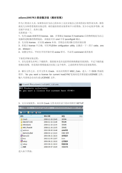
2、解压文件之后,打开文件夹Crack,双击应用程序MSC_Calc,进入一个DOS界面的程序,"do you want a license for current host(Y/N)"是询问是否要创建LICENSE文件,输入Y,系统会自动生成LICENSE文件。
3、完全安装软件:双击和Crack文件夹同目录下的应用程序SETUP进入如下界面:先点LICENSE,进入,系统会自动在C盘下面建立文件夹MSC.Software,最后需要导入li cense.dat文件,马上把在步骤2中生成的license.dat复制到目录:C:\MSC.Software\MS C.Licensing\10.8.6下,然后把这个文件导入,OK!等一下,进入上面图片上显示的MD Ad ams下完全安装软件,过程中视自己的需要安装模块,再一次导入license文件后安装完成!4、设置系统变量进入计算机的属性→高级系统设置→环境变量→系统变量设置系统变量:变量名和变量值如下图所示确定,然后退出变量设置!5、flexlm配置实用程序:开始-程序-MSC.Software-MSC.Licensing10.8.6-FLEXlm Config uration Utility,进入下面界面点configurationg using Service 选择MSC Licensing 10.8.6;然后点击Config Service,进入下面界面:Service name选择MSC Licensing 10.8.6,下面三个请Browse,在如图框的C盘安装目录下导入相应的lmgrd.exe文件、license文件,第三个可以不管跳过;选中最下面的两个备选项,然后Save Service,接下来点击Start/Stop/Reread,进入下面的界面:先点击Stop Server,再点击Start Server,最下面会显示run succesful,运行成功!此时基本上就完全成功了!但是下面这最后一点确实最最重要的!6、这一点很重要,这时候安装已经完成,但是在启动之前必须重启电脑!重新启动后,把开始菜单里的ADAMS各程序VIEW、slover等创建快捷方式到桌面,双击快捷方式,就可以运行程序了!7、最后要说明的是本人的操作系统是VISTA!。
Adams软件后置处理
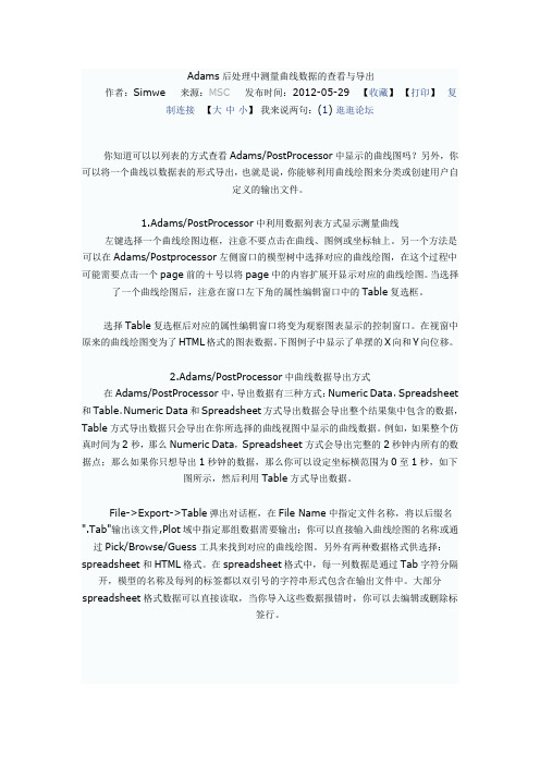
Adams后处理中测量曲线数据的查看与导出作者:Simwe 来源:MSC发布时间:2012-05-29 【收藏】【打印】复制连接【大中小】我来说两句:(1) 逛逛论坛你知道可以以列表的方式查看Adams/PostProcessor中显示的曲线图吗?另外,你可以将一个曲线以数据表的形式导出,也就是说,你能够利用曲线绘图来分类或创建用户自定义的输出文件。
1.Adams/PostProcessor中利用数据列表方式显示测量曲线左键选择一个曲线绘图边框,注意不要点击在曲线、图例或坐标轴上。
另一个方法是可以在Adams/Postprocessor左侧窗口的模型树中选择对应的曲线绘图,在这个过程中可能需要点击一个page前的+号以将page中的内容扩展开显示对应的曲线绘图。
当选择了一个曲线绘图后,注意在窗口左下角的属性编辑窗口中的Table复选框。
选择Table复选框后对应的属性编辑窗口将变为观察图表显示的控制窗口。
在视窗中原来的曲线绘图变为了HTML格式的图表数据。
下图例子中显示了单摆的X向和Y向位移。
2.Adams/PostProcessor中曲线数据导出方式在Adams/PostProcessor中,导出数据有三种方式:Numeric Data,Spreadsheet 和Table。
Numeric Data和Spreadsheet方式导出数据会导出整个结果集中包含的数据,Table方式导出数据只会导出在你所选择的曲线视图中显示的曲线数据。
例如,如果整个仿真时间为2秒,那么Numeric Data,Spreadsheet方式会导出完整的2秒钟内所有的数据点;那么如果你只想导出1秒钟的数据,那么你可以设定坐标横范围为0至1秒,如下图所示,然后利用Table方式导出数据。
File->Export->Table弹出对话框,在File Name中指定文件名称,将以后缀名".Tab"输出该文件,Plot域中指定那组数据需要输出;你可以直接输入曲线绘图的名称或通过Pick/Browse/Guess工具来找到对应的曲线绘图。
ADAMS后处理中数据及图形导出方法
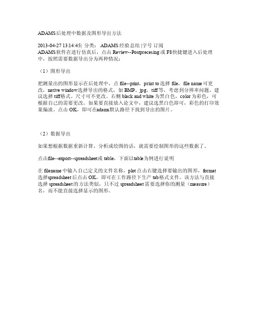
ADAMS后处理中数据及图形导出方法2013-04-27 13:14:45| 分类: ADA MS经验总结 |字号订阅A DAMS软件在进行仿真后,点击Revie w--Po stpre cesin g或F8快捷键进入后处理中,按照需要数据导出分为两种情况:(1)图形导出把测量出的图形显示在后处理中,点file--pri nt,pr int t o选择fi le,fi le na me可更改,nati ve wi ndow选择导出的格式,如BM P、jpg、tiff等,考虑到分辨率问题,建议选择tiff格式。
尺寸可不更改。
右侧blac k and whit e为黑白色,colo r为彩色,可根据自己的需要更改。
如果要直接放入论文中,建议选黑白色即可,彩色的打印效果偏淡。
点击OK,即可在a dams默认路径下找到导出的图片。
(2)数据导出如果想根据数据重新计算、分析或绘图的话,就需要绘制图形的这些数据了。
点击f ile--expor t--sp reads heet或table,下面以t able为例进行说明在fi lenam e中输入自己定义的文件名称,p lot点击右键选择要输出的图形,form at 选择s pread sheet后点击OK,即可在工作路径下生产tab格式文件。
该方法与直接选择spr eadsh eet的方法类似,只不过spr eadsh eet需要选择你的测量(mea sure)名,而不能直接选择显示的图形。
。
ADAMS系统测量与仿真和仿真后处理
对象 结构 关系
栏
特性 编辑 区
工具条
后处理程序窗口
后处理的绘图 区
菜单栏 页面操 作区
控制面 板区 状态 栏
2、仿真模型的调入和仿真重 现
仿真模型调入:
I)激活拟显示虚拟样机仿真过程的屏 幕视窗,然后将鼠标置于视窗上, 打开弹出式菜单。
2)选择Load Animation命令,调入 ADAMS/View的仿真计算结果,可 以在屏幕上看见已经调入的样机。
名称 测量零件 测量特征 测量分量
测 量 构Ⅰ 件 对 话 框
Selected Object参数表示构件、运 动副、力、运动、点或标记等各种对
象的测量;
Point—to—Point参数表示两点之间 的相对运动测量;
Orientation参数表示坐标系标记方向 的测量;
Range 参数表示已定义的测量的统计值 ,例如:平均值、最大值等;
页的操作
操作工具
后
前新
删
翻
翻建
除
视窗的操作
视窗布置 选择视窗 放大视窗 转移视窗内容 删除视窗内容
对象结构关系及其转性编辑
Modeling项包括与仿真样机 有关的各种对象类型,例如 :构件、运动副、作用力等
Plotting项包括与绘制 数据曲线图有关的各种 对象类型,例如:曲线
、标题等。
重现仿真过程
数据曲线自变量坐标轴的选择
在控制面板右侧 的自变量轴选择 区(Independent
Axis),选择 Data项
在弹出的自变量 轴浏览对话框, 选择自变量轴(X 轴)的变量,然
后选择OK
修改坐标轴的特性
特性:坐标轴 的范围、颜色 、坐标刻度、 坐标刻度标记 、坐标标题和
adams后处理学习资料
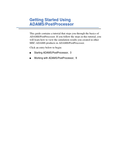
Getting Started UsingADAMS/PostProcessorThis guide contains a tutorial that steps you through the basics of ADAMS/PostProcessor. If you follow the steps in this tutorial, you will learn how to view the simulation results you created in other MSC.ADAMS products in ADAMS/PostProcessor.Click an entry below to begin:■Starting ADAMS/PostProcessor,3■Working with ADAMS/PostProcessor,9Getting Started Using ADAMS/PostProcessor 2CopyrightThe information in this document is furnished for informational use only, may be revised from time to time, and should not be construed as a commitment by MSC.Software Corporation. MSC.Software Corporation assumes no responsibility or liability for any errors or inaccuracies that may appear in this document.Copyright InformationThis document contains proprietary and copyrighted information. MSC.Software Corporation permits licensees of MSC.ADAMS software products to print out or copy this document or portions thereof solely for internal use in connection with the licensed software. No part of this document may be copied for any other purpose or distributed or translated into any other language without the prior written permission of MSC.Software Corporation.Copyright © 2004 MSC.Software Corporation. All rights reserved. Printed in the United States of America. TrademarksADAMS, EASY5, MSC, MSC., MSC.ADAMS, MSC.EASY5, and all product names in the MSC.ADAMS Product Line are trademarks or registered trademarks of MSC.Software Corporation and/or its subsidiaries.NASTRAN is a registered trademark of the National Aeronautics Space Administration. MSC.Nastran is an enhanced proprietary version developed and maintained by MSC.Software Corporation. All other trademarks are the property of their respective owners.Government UseUse, duplication, or disclosure by the U.S. Government is subject to restrictions as set forth in FAR 12.212 (Commercial Computer Software) and DFARS 227.7202 (Commercial Computer Software and Commercial Computer Software Documentation), as applicable.Starting ADAMS/PostProcessorOverviewWe’ve provided a tutorial that steps you through the basics ofADAMS/PostProcessor. If you follow the steps in this tutorial, youwill learn how to view the simulation results you created in otherMSC.ADAMS products in ADAMS/PostProcessor. The sections inthe chapter are:■What You Will Do in the Tutorial, 4■Starting ADAMS/PostProcessor, 4■Loading the Simulation Results, 5The tutorial takes about 20 minutes to complete.Getting Started Using ADAMS/PostProcessor 4Starting ADAMS/PostProcessorWhat You Will Do in the TutorialIn the tutorial, you’ll learn how to:1View reports.2Play an animation of simulation data, including animating the results of a clearance study.3Display simulation results as both xy plots and tables.4View animations and plots simultaneously.Starting ADAMS/PostProcessorYou can run ADAMS/PostProcessor as a stand-alone product or from within other MSC.ADAMS products, such as ADAMS/View, ADAMS/Car, or ADAMS/Engine. The following instructions explain how to start ADAMS/PostProcessor in stand-alone mode. It also explains how to start any add-ons or plugins to ADAMS/PostProcessor. Currently, the only plugin is for ADAMS/Durability.To start ADAMS/PostProcessor stand-alone in UNIX:1At the command prompt, enter the command to start the MSC.ADAMS Toolbar, and then press Enter. The standard command that MSC.Softwareprovides is adams x, where x is the version number, for example, adams2005represents MSC.ADAMS 2005.The MSC.ADAMS Toolbar appears.2Click the ADAMS/PostProcessor tool .For more information on the MSC.ADAMS Toolbar, see the guide, Runningand Configuring MSC.ADAMS on UNIX.To start ADAMS/PostProcessor stand-alone in Windows:■From the Start menu, point to Programs, point to MSC.Software, point to MSC.ADAMS 2005, point to APostProcessor, and then select ADAMS -PostProcessor.For more information on running MSC.ADAMS products from the Startmenu, see the guide, Running MSC.ADAMS on Windows.Getting Started Using ADAMS/PostProcessorStarting ADAMS/PostProcessor5Loading the Simulation ResultsWe’ve provided you with simulation results that you can use to learn the basics of ADAMS/PostProcessor. The simulation results are in two files:■ppt_gs.gra - Graphics file containing information that enablesADAMS/PostProcessor to animate a model of a suspension. It also containstime-dependent data describing the position and orientation of each part in themodel.■ppt_gs.req - Request file containing information that enablesADAMS/PostProcessor to create plots of simulation results. It containsinformation about the various data requested and time history of all the requestvalues.In this tutorial, you import these files through the command file ppt_gs.cmd. The command file also sets up several pages containing animations and plots. In addition, it runs a clearance study as it loads the files.The files are located in the directory /install_dir/ppt/examples, where install_dir is the directory where you installed the MSC.ADAMS products. To get the results into ADAMS/PostProcessor, you need to copy the files to your working directory and import the command file.To copy the files:■In the directory /install_dir/ppt/examples, copy the following files to your working directory:■ppt_gs.cmd■ppt_gs.req■ppt_gs.gra■ppt_gs.html■ppt_gs.pngGetting Started Using ADAMS/PostProcessor 6Starting ADAMS/PostProcessor To import ppt_gs.cmd:1From the File menu, point to Import, and then select Command File.2Right-click the File Name box, and then select Browse.3Use the Open dialog box to find the file ppt_gs.cmd, and then select OK.4In the File Import dialog box, select OK.The command file that you imported into ADAMS/PostProcessor creates several pages containing reports, animations, and plots. It also runs a clearance study.Familiarizing Yourself with ADAMS/PostProcessorADAMS/PostProcessor has four modes:animation, plotting, reports, and 3D plotting (only available with ADAMS/Vibration and ADAMS/Engine data). It switches its modes automatically depending on the contents of the active viewport. For example, the tools in the Main toolbar change if you load an animation or a plot into a viewport.Figure1 on page 7shows the ADAMS/PostProcessor window. The elements shown are common to all modes.Getting Started Using ADAMS/PostProcessorStarting ADAMS/PostProcessor 7Figure 1. ADAMS/PostProcessor WindowThe elements in the ADAMS/PostProcessor window are:■Menu bar - Contains the headings of each menu. ■Main toolbar - Displays commonly used tools for working with animations, plotting results, and reports. It changes depending on whether you are viewinganimations, plots, or reports.■Treeview - Displays a hierarchical list of the models and pages. The tree is especially useful for selecting and identifying objects.■Property editor - Lets you change the properties of selected objects.■Status toolbar - Displays information messages and prompts while you work.■Page - Displays the current page. Each page can display up to six rectangular areas or viewports in which you can place animations and plots.■Viewports - Rectangular areas that display different views of plots, animations, or reports.■Dashboard - Provides functions for controlling animations or plotting results.Status toolbarGetting Started Using ADAMS/PostProcessor 8Starting ADAMS/PostProcessorWorking with ADAMS/PostProcessor OverviewThis chapter steps you through working with three of theADAMS/PostProcessor modes: reports, animations, and plotting:■Displaying Reports, 10■Working with Animations, 10■Working with Plots, 12■Viewing Plots and Animations Simultaneously, 17■The Next Step, 17Getting Started Using ADAMS/PostProcessor 10Working with ADAMS/PostProcessor Displaying ReportsThe first page, which ADAMS/PostProcessor displays by default, is a page p1_report, which displays a report of the pages that the command file you imported created. As you can see from the report, you can use simple HTML tags and bitmapped images to display information about the animations and plots in ADAMS/PostProcessor. You can also display reports of clearance studies. For more information on displaying reports and the HTML tags that ADAMS/PostProcessor supports, see the ADAMS/PostProcessor online help.Working with AnimationsNow you’ll review the animation you loaded with the clearance study results that ADAMS/PostProcessor just performed. You’ll view the animations in different ways, including interactively setting the speed at which ADAMS/PostProcessor runs the animations.Viewing an AnimationThe animation that you will view is stored on the page named p2_clearance.To select the animation page:■In the treeview, select p2_clearance.ADAMS/PostProcessor switches to animation mode and displays the first frame of the animation. All the elements in the dashboard change to those forcontrolling animations. The pull-down menu at the top ofADAMS/PostProcessor to the right of the toolbar also changes to Animation toindicate the current mode.Notice the red and green lines in the animation:■The green line tracks the distance between the right wheel (PART_21) and the steering wheel (PART_10).■The red line tracks the distance between the left wheel (PART_22) and the steering wheel (PART_10).Working with ADAMS/PostProcessor11 To run the animation:■At the top of the dashboard, select the Play tool.Notice that ADAMS/PostProcessor continuously plays the animation. You can also set ADAMS/PostProcessor so that it plays the animation only once or plays the animation forward and then backward.To set the animation to play only once:1On the dashboard, select Animation, if necessary.2Set Loop to Once.Interactively Playing the AnimationTo help you investigate the results of a simulation, you can play animation frames forwards and backwards, rewind to an earlier frame, or play only a portion of the animation. In this tutorial, you’ll interactively play the animation by dragging the animation slider.To interactively play the animation:1To rewind the animation, select the Reset tool.2At the top of the dashboard, drag the slider bar back and forth to watch how the animation plays backwards and forwards at the speed at which you drag the slider.Working with PlotsADAMS/PostProcessor also plots the results of simulations so you can interpret the performance of your design. In this section, you’ll view pages with plots on them, modify the plots, and create your own plots.Viewing Pages of PlotsA page, called p3_plots, already exists that contains several plots that you will view. You’ll first view all the plots and then you’ll quickly zoom in on just one of the plots. Notice that p3_plots in the lower left corner is a plot that ADAMS/PostProcessor has displayed as a table. In the treeview, it is still listed as a plot.To view the plotting page:1In the treeview, select p3_plots.ADAMS/PostProcessor switches to plotting mode and displays the plots.2Click the plot in the upper right corner of the window and, from the Main toolbar,select the Expand View tool.ADAMS/PostProcessor displays only the selected plot.3To return to viewing all the plots, select the Expand View tool again.Working with ADAMS/PostProcessor13Modifying Plotting ObjectsYou can tailor the appearance of plots to help you identify the information in the plot more effectively or to make the plot ready for a presentation. In this section, you’ll turn off the grid lines and change the line style of the curves of one of the plots.Displaying the Table as a PlotBefore you begin to change the look of plots, you’ll change the plot displayed as a table (plot_4) back to being an xy plot.To change the table to a plot:1In the viewport, select plot_4.2In the property editor, clear the selection of Table.Turning Off Grid LinesIn ADAMS/PostProcessor, plots contain primary and secondary grid lines that serve as visual guides for inspecting curves. Primary grid lines appear at all major unit sections. Secondary grid lines appear at specified intervals between the primary grid lines. In this section, you’ll turn off the visibility of the grid lines in one plot. You’ll do this by selecting the plot and then editing its properties in the Property Editor.To turn off primary lines:1Click the border of the plot in the upper right corner.Notice that the viewport border turns red to indicate that you’ve selected it. Inaddition, the treeview highlights the plot. You are now ready to edit the properties of the selected plot.2In the property editor, select Grid.3Clear the selection of Visible.4In the property editor, select the right arrow key to display more tabs.5Select 2nd Grid.6Clear the selection of Visible.Changing Color and Line Style of All CurvesNow you’ll use the treeview to learn how to modify a group of common objects all at once. In this example, you’ll change the line styles of all the curves in the plots on page p3_plots.To change all curves:1To expand the treeview so it displays all plots on the page p3_plots, in the treeview, click the plus sign (+) in front of the page p3_plots.2Now click the plus sign (+) in front of each plot on the page p3_plots to see all the objects in the plots.3In the treeview, hold down the Ctrl key, and select each curve on page p3_plots.4In the property editor, from the Line Style box, select Dash.All the curves change to dashed lines.To reset the filter to show all objects:■Right-click the background of the treeview, point to Type Filter, and then select All.Creating New PlotsYou can also create your own plots as shown in the next steps.Creating a PageBefore you can create a plot, you need to create a page for it.To create a page:■On the Main toolbar, select the New Page tool.Because you are in plotting mode, ADAMS/PostProcessor displays plots onwhich to add data. If you were in animation mode, ADAMS/PostProcessorwould display empty viewports for loading animations.To set the layout of the page so it contains two viewports:■In the Main toolbar, right-click the Page Layout tool stack, and then select .Working with ADAMS/PostProcessor15Adding Data to the PlotNow that you have a new page, you can display some curves on it. In plot mode, the dashboard contains the numeric results of loaded simulation results. It displays the objects, measures, requests, and result sets from ADAMS simulations and any results from clearance studies. The results that you have available depend on the output that you requested from your MSC.ADAMS product. For information on the different results you can generate, see your MSC.ADAMS product online help.In this tutorial, you’ll use requests, which provide standard displacement, velocity, acceleration, or force information that will help you investigate the results of your simulation. Requests also let you define other quantities (such as pressure, work, energy, momentum, and more) that you want generated during a simulation.To add a curve to the plot, select the following from the dashboard:1In the dashboard, in the Request box, select REQ1080 TOE CASTER CAMBER (FRONT).2In the Component box, select X, Y, and Z.3Select Add Curves.4Now add more curves by selecting different data from the dashboard and selecting Add Curves.Surfing Through DataIn the previous section, for each request you selected, ADAMS/PostProcessor added new curves to your plot. You can also plot your data without accumulating curves on your plot. This is called surfing. It is convenient for quickly looking at different data.To quickly add data without creating new curves:1Select the plot on the right.2In the dashboard, select Surf.3Select the data that you’d like to view, as explained earlier.You’ll notice that each time you select data, ADAMS/PostProcessor replaces the existing curves with new curves.Modifying a CurveNot only can you view data in ADAMS/PostProcessor, but you can also change and enhance it. In this tutorial, you’ll change the mathematical expression that creates a curve. To change a curve:1Click a curve on the plot on the left.2At the top of the dashboard, select Math.The dashboard displays the mathematical expressions used to calculate the curve. 3In the Y Expression box, change the mathematical expression, and then select Apply.You can change it in different ways. For example, enter a negative sign(-) in front of the expression to invert the values or multiply the expression by 3.Working with ADAMS/PostProcessor17Viewing Plots and Animations SimultaneouslyYou can place plots and animations together on the same page, and you can also run the animation and see ADAMS/PostProcessor track the corresponding data on the plot as the animation plays.To view plots and animations together:1In the treeview, select the page p4_combined.ADAMS/PostProcessor displays a page containing both animations and plots.2At the top of the dashboard, select the Play tool.ADAMS/PostProcessor plays the animation and displays a line on the plot at the same data point that the animation is displaying.The Next StepYou completed a few of the most common operations in ADAMS/PostProcessor for working with simulation results. Now use the ADAMS/PostProcessor online help as a reference to the many features of ADAMS/PostProcessor.。
- 1、下载文档前请自行甄别文档内容的完整性,平台不提供额外的编辑、内容补充、找答案等附加服务。
- 2、"仅部分预览"的文档,不可在线预览部分如存在完整性等问题,可反馈申请退款(可完整预览的文档不适用该条件!)。
- 3、如文档侵犯您的权益,请联系客服反馈,我们会尽快为您处理(人工客服工作时间:9:00-18:30)。
b1 + b 2 s + b3 s + ... + b m s H (s) = 2 n a1 + a 2 s + a 3 s + ... + a n s
2 m
FFT
Main menu->plot->FFT
FFT
• • •
FFTMAG FFT算法得到的幅值。 FFTPHASE FFT算法得到的相位角 PSD 确定信号频率组成中的能量分布
• •
曲线
动画
ADAMS / PostProcessor Window
Toolbar
• • •
主工具箱: 主工具箱: 曲线编辑工具箱: 曲线编辑工具箱: 统计工具箱: 统计工具箱:
曲线编辑工具箱
• • • • • •
曲线相加、 绝对值,比例, 曲线相加、减、乘,绝对值,比例,负值 曲线插值、偏移、 曲线插值、偏移、对准 微分、积分 微分、 样条、显示数据标记 样条、 滤波:低通、高通、带通、带阻 滤波:低通、高通、带通、 FFT
•
Butterworth filter - butter() in MATLAB
1 H ( s) H (− s) = , N为滤波器阶次 2N 1 + ( s jω )
•
Transfer function - A filter you define by directly specifying the coefficients of a transfer function.
练习用文件
•
将ADAMS 11.0 \ PPT \Example目录中的文件拷贝到你的 Example目录中的文件拷贝到你的 工作目录: 工作目录: 汽车悬架系统仿真的后处理的文件: 汽车悬架系统仿真的后处理的文件: ppt_gs.gra – ppt_gs.req – ppt_gs.cmd – 包含模型、仿真结果的图形文件。 包含模型、仿真结果的图形文件。 Request 文件 包含模型、仿真结果的命令文件。 包含模型、仿真结果的命令文件。
Bode 图
Main menu->plot->Bode
Bode 图
• •
转换函数法: 转换函数法:
» Transfer Functions Coefficient » TFSISO (ADAMS 格式单输入、单输出传递函数) 格式单输入、单输出传递函数
矩阵法
» ADAMS Linear State Matrix:用线性化模型的状态矩 : 阵 » ADAMS Matrix
•
输入输出信号对法: 输入输出信号对法:
» Time Domain Measure: 用测量定义系统输入、输出 用测量定义系统输入、 » Time Domain Result set Components:用仿真输出 : 定义系统
• •
File Import:将文件装入后处理。 Import:将文件装入后处理。 进行各种操作练习。 进行各种操作练习。
数据处理 • Filtering Curve Data
Performing FFT Functions Constructing Bode Plots
滤波 Filtering
统计工具箱
•
实时显示数据点x, y 坐标、斜率 坐标、 实时显示数据点
» X Y Slope
•
最大值、最小值、平均值、均方根值 最大值、最小值、平均值、
» Min Max Avg RMS
动画显示、控制和输出
• • • • •
动画 设置选项:光标、坐标系、标题等 设置照相机 记录动画 从叠显示多个动画
ADAMS/PPT
Post Processor 后处理器
后处理
•
Debugging - ADAMS/PostProcessor 通过动 图形帮助你调试模型。 画、图形帮助你调试模型。 Validating – 输入物理样机的数据和曲线图与 仿真结果比较,以评价仿真的有效性。 仿真结果比较,以评价仿真的有效性。 Refining – 比较不同的仿真结果,以确定更 比较不同的仿真结果, 好的模型。 好的模型。 Presenting Results – 生动、形象地演示仿 生动、 真结果,还可产生动画短片,用于其它演示。 真结果,还可产生动画短片,用于其它演示。
启动 PPT
• •
Start menu Programs ADAMS 11.0 APostProcessor PostProbox PPT 图标
ADAMS / PPT 输入文件
• •
ADAMS/View: command (.cmd) 模型文件 ADAMS/Solver: Dataset (.adm) – 用ADL语言的模型文件 语言的模型文件 Analysis: Graphics – .gra Request – .req Results –- .res Numeric data: ASCII 文件 Wavefront objects, Stereolithography, render, and shell:Polygonal representation of surfaces.