计量经济学导论第四版英文完整教学课件
合集下载
《计量经济学导论》ch4
Multiple Regression Analysis: Inference
Discussion of the normality assumption The error term is the sum of „many“ different unobserved factors Sums of independent factors are normally distributed (CLT) Problems: • How many different factors? Number large enough? • Possibly very heterogenuous distributions of individual factors • How independent are the different factors? The normality of the error term is an empirical question At least the error distribution should be „close“ to normal In many cases, normality is questionable or impossible by definition
Sampling distributions of the OLS estimators The OLS estimators are random variables We already know their expected values and their variances However, for hypothesis tests we need to know their distribution In order to derive their distribution we need additional assumptions Assumption about distribution of errors: normal distribution
2024版计量经济学全册课件(完整)pptx

REPORTING
2024/1/28
23
EViews软件介绍及操作指南
EViews软件概述
EViews是一款功能强大的计量经济学 软件,提供数据处理、统计分析、模型
估计和预测等功能。
统计分析与检验
2024/1/28
详细讲解EViews中的统计分析工具, 包括描述性统计、假设检验、方差分
析等。
数据导入与预处理 介绍如何在EViews中导入数据,进行 数据清洗、转换和预处理等操作。
随着大数据时代的到来,机器学 习算法在数据挖掘、预测和分类 等方面展现出强大的能力,为计 量经济学提供了新的研究工具和 方法。
机器学习在计量经济 学中的应用领域
机器学习在计量经济学中的应用 领域广泛,如变量选择、模型选 择、非线性模型估计、高维数据 处理等。
机器学习在计量经济 学中的常用算法
机器学习在计量经济学中常用的 算法包括决策树、随机森林、支 持向量机(SVM)、神经网络等。 这些算法可以用于分类、回归、 聚类等任务,提高模型的预测精 度和解释力。
面板数据特点
同时具有时间序列和截面数据的特征,能够提供更多的信息、更多的变化、更少共 线性、更多的自由度和更高的估计效率。
2024/1/28
20
固定效应模型与随机效应模型
固定效应模型(Fixed Effects Model)
对于特定的个体而言,其截距项是固定的,不随时间变化而变化。
随机效应模型(Random Effects Mode…
经典线性回归模型
REPORTING
2024/1/28
7
一元线性回归模型
模型设定与参数估计
介绍一元线性回归模型的基本形式, 解释因变量、自变量和误差项的含义, 阐述最小二乘法(OLS)进行参数估 计的原理。
计量经济学(英文版)精品PPT课件
(4.3a)
Expand and multiply top and bottom by n:
b2
=
nSxiyi - Sxi Syi nSxi2-(Sxi) 2
(4.3b)
Variance of b2
4.12
Given that both yi and ei have variance s2,
the variance of the estimator b2 is:
4. cov(ei,ej) = cov(yi,yj) = 0 5. xt c for every observation
6. et~N(0,s 2) <=> yt~N(b1+ b2xt,
The population parameters b1 and b2 4.4 are unknown population constants.
b2
+
nSxiEei - Sxi SEei nSxi2-(Sxi) 2
Since Eei = 0, then Eb2 = b2 .
An Unbiased Estimator
4.8
The result Eb2 = b2 means that the distribution of b2 is centered at b2.
4.6
The Expected Values of b1 and b2
The least squares formulas (estimators) in the simple regression case:
b2 =
nSxiyi - Sxi Syi nSxi22 -(Sxi) 2
b1 = y - b2x
第1讲导论整理ppt
21
理论的创立
Frisch
经
典
建立第1个应用模型
Tinbergen
计
量 经
建立投入产出模型
Leontief
济
学
发展应用模型
Klein
发展数据基础
Stone
建立概率论基础
Haavelmo
22
The Bank of Sweden Prize in Economic Sciences in Memory of Alfred Nobel 2000
31
参数估计
选择适当的方法和软件估算出模型的参数
国家组别
低收入 中等收入 高收入 世界平均
人均GDP 平均受教育年限 明瑟收益率
(美元)
(年)
(%)
375
7.6
10.9
3025
8.2
10.7
23463
9.4
7.4
9160
8.3
9.7
•1998年数据
32
参数估计
我国城镇地区明瑟收益率
明 瑟 收 益 率 (%)
"for his clarification of the probability theory foundations of econometrics and his analyses of
simultaneous economic structures"
Trygve Haavelmo Norway
时间序列: 自回归条件异方差 —现代金融计量
Heckman McFadden
Granger Engle
27
三、计量经济分析的步骤
1. 建立理论模型和计量模型 2. 收集样本数据 3. 参数估计 4. 假设检验 以教育收益率为例
计量经济学导论PPT课件

• 必须掌握一种应用软件(Spss或Eviews),注意课堂和实 验的软件应用演示。
第一章 导 论
什么是计量经济学 计量经济学研究的步骤 计量经济学模型与数据 计量经济学的产生与发展
第一节 什么是计量经济学
◆ 计量经济学的定义 ◆ 计量经济学与其它学科的关系 ◆ 计量经济学的内容体系
一、计量经济学的定义
▼ 第一届诺贝尔经济学奖得主挪威经济学家R. Frisch将计量经济学定义为经济理论、统计学和 数学的结合;
▼ P.A.Samuelson、T.C.Koopmans、R.Stone将 计量经济学定义为“应用合适的方法对经济理论 和观察到的事实加以联系和推导,对现实经济现 象进行定量分析”。
一、计量经济学的定义
应用计量经济学——运用理论计量经济学所提供的理论
与方法研究 特定领域的具体经济活动的数量关系,侧重于建 立与应用模型过程中的实际问题的处理,除依赖理论计量经 济学外,需要依赖经济理论建立模型,根据具体的经济数据 进行分析、预测、评价等。
宏观计量经济学与微观计量经济学
区分依据:
对应于宏观经济学与微观经济学的划分
(对数学的应用)
第一,对非线性函数进行线性转化的方法和技巧,是 数学在计量经济学中的应用
第二,任何的参数估计归根结底都是数学运算,较复 杂的参数估计方法,或者较复杂的模型的参数估计, 更需要相当的数学知识和数学运算能力
第三,在计量经济理论和方法的研究方面,需要用到 许多的数学知识和原理
计量经济学与其它学科的区别
个人消费C
GDP
1980
2447.1
3776.3
1981
2476.9
3843.1
1982
2503.7
《计量经济学英文版》课件

2 ARMA模型
介绍ARMA模型的基本原 理和参数估计方法,以及 ARMA模型在经济数据分 析中的应用。
3 GARCH模型
讲解GARCH模型的原理 和估计方法,以及 GARCH模型在金融市场 波动预测中的应用。
计量经济模型的应用
金融市场分析
应用计量经济模型进行金融市 场的预测和分析。
政策评估
利用计量经济模型评估政策的 效果和影响。
面板数据模型
1
面板数据概述
介绍面板数据的特点和应用领域,以及面板数据模型的基本概念。
2
固定效应模型
讲解固定效应模型的估计和推断方法,以及固定效应模型的优缺点。
3
随机效应模型
介绍随机效应模型的估计和推断方法,以及随机效应模型与固定效应模型的比较。
时间序列模型
1 时间序列数据基本特
征
描述时间序列数据的基本 特征,如趋势、季节性和 周期性。
《计量经济学英文版》 PPT课件
本课程介绍了计量经济学的基本概念和分析方法。涵盖了经济数据与计量分 析、经典线性回归模型、面板数据模型、时间序列模型和计量经济模型的应 用。
课程概述
本节将概述本课程的内容,包括学习目标和涵盖的主要内容。通过本课程的学习,您将掌握计量经济学的基本 理论和实际应用。
经济数据与计量分析
企业ቤተ መጻሕፍቲ ባይዱ策
运用计量经济模型辅助企业的 决策制定。
总结
通过本课程的学习,您将获得计量经济学分析的基本知识和技能,能够应用计量经济模型进行实证研究,并在 实际问题中运用计量经济学的方法和工具。
• 经济数据的概念与特点 • 统计概率基础 • 经济计量分析的目的与意义
经典线性回归模型
普通最小二乘法
(2024年)完整版李子奈计量经济学版第四版课件

• 二阶段最小二乘法(2SLS):二阶段最小二乘法是一种常用的联立方程模型估 计方法。该方法首先对每个方程进行最小二乘估计,得到每个方程的残差;然 后使用这些残差作为解释变量,对所有方程进行再次估计。这种方法可以消除 方程之间的相互影响,得到一致的参数估计量。
• 三阶段最小二乘法(3SLS):三阶段最小二乘法是对二阶段最小二乘法的改进。 该方法在第二阶段估计时,不仅考虑了残差作为解释变量,还考虑了其他所有 内生变量的估计值作为解释变量。这样可以进一步提高参数估计量的效率。
在社会科学领域,这些方法可用于分析人口 统计数据、经济指标等,揭示社会经济现象 背后的复杂关系。
2024/3/26
30
THANKS
感谢观看
2024/3/26
31
多重共线性的检验
相关系数矩阵法、方差膨胀因子 法、条件指数法等。
14
04
时间序列计量经济学模型
Chapter
2024/3/26
15
时间序列基本概念与性质
01
02
03
时间序列定义
按时间顺序排列的一组数 据,反映现象随时间变化 的发展过程。
2024/3/26
时间序列构成要素
现象所属的时间(年、季、 月、日等)和反映现象在 各个时间上的统计指标数 值。
28
半参数回归分析方法
部分线性模型
模型中既包含参数部分也包含非参数部分,参数部分用于描述主要 影响因素,非参数部分用于捕捉其他未知影响因素。
单指标模型
通过投影寻踪方法将高维数据降维到一维,然后利用非参数方法进 行回归分析。
变系数模型
模型系数随着某个或多个变量的变化而变化,可以灵活捕捉变量间的 动态关系。
不可识别的情况 当联立方程模型中的某个方程不能被任何其他方程所替代 时,该方程就是不可识别的。此时,无法对该方程的参数 进行一致估计。
计量经济学导论 PPT ch04
0 1
x1
x2
Economics 20 - Prof. Anderson 4
Normal Sampling Distributions
Under the CLM assumptions, conditional on the sample values of the independent variables β ~ Normal β , Var β , so that
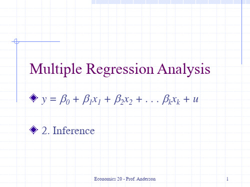
Multiple Regression Analysis
y = β0 + β1x1 + β2x2 + . . . βkxk + u 2. Inference
Economics 20 - Prof. Anderson
1
Assumptions of the Classical Linear Model (CLM)
2
Economics 20 - Prof. Anderson 6
The t Test (cont)
Knowing the sampling distribution for the standardized estimator allows us to carry out hypothesis tests Start with a null hypothesis For example, H0: βj=0 If accept null, then accept that xj has no effect on y, controlling for other x's
Economics 20 - Prof. Anderson 2
CLM Assumptions (cont)
Under CLM, OLS is not only BLUE, but is the minimum variance unbiased estimator We can summarize the population assumptions of CLM as follows y|x ~ Normal(β0 + β1x1 +…+ βkxk, σ2) While for now we just assume normality, clear that sometimes not the case Large samples will let us drop normality
x1
x2
Economics 20 - Prof. Anderson 4
Normal Sampling Distributions
Under the CLM assumptions, conditional on the sample values of the independent variables β ~ Normal β , Var β , so that
Multiple Regression Analysis
y = β0 + β1x1 + β2x2 + . . . βkxk + u 2. Inference
Economics 20 - Prof. Anderson
1
Assumptions of the Classical Linear Model (CLM)
2
Economics 20 - Prof. Anderson 6
The t Test (cont)
Knowing the sampling distribution for the standardized estimator allows us to carry out hypothesis tests Start with a null hypothesis For example, H0: βj=0 If accept null, then accept that xj has no effect on y, controlling for other x's
Economics 20 - Prof. Anderson 2
CLM Assumptions (cont)
Under CLM, OLS is not only BLUE, but is the minimum variance unbiased estimator We can summarize the population assumptions of CLM as follows y|x ~ Normal(β0 + β1x1 +…+ βkxk, σ2) While for now we just assume normality, clear that sometimes not the case Large samples will let us drop normality
计量经济学导论-ch3 36页PPT文档
Example: Wage equation
Now measures effect of education explicitly holding experience fixed
All other factors…
Hourly wage
Years of education
Labor market experience
© 2013 Cengage Learning. All Rights Reserved. May not be scanned, copied or duplicated, or posted to a publicly accessible website, in whole or in part.
© 2013 Cengage Learning. All Rights Reserved. May not be scanned, copied or duplicated, or posted to a publicly accessible website, in whole or in part.
© 2013 Cengage Learning. All Rights Reserved. May not be scanned, copied or duplicated, or posted to a publicly accessible website, in whole or in part.
Multiple Regression Analysis: Estimation
Definition of the multiple linear regression model
„Explains variable in terms of variables
伍德里奇计量经济学导论第四版
课
后
(ii) plim(W1) = plim[(n – 1)/n] ⋅ plim( Y ) = 1 ⋅ µ = µ. plim(W2) = plim( Y )/2 = µ/2. Because plim(W1) = µ and plim(W2) = µ/2, W1 is consistent whereas W2 is inconsistent.
m
(ii) This follows from part (i) and the fact that the sample average is unbiased for the population average: write
W1 = n −1 ∑ (Yi / X i ) = n −1 ∑ Z i ,
i =1 i =1
n
n
where Zi = Yi/Xi. From part (i), E(Zi) = θ for all i. (iii) In general, the average of the ratios, Yi/Xi, is not the ratio of averages, W2 = Y / X . (This non-equivalence is discussed a bit on page 676.) Nevertheless, W2 is also unbiased, as a simple application of the law of iterated expectations shows. First, E(Yi|X1,…,Xn) = E(Yi|Xi) under random sampling because the observations are independent. Therefore, E(Yi|X1,…,Xn) = θ X i and so
伍德里奇计量经济学导论第四版
i =1 n
ˆ= 5.8125, and ∑ (xi – x )2 = 56.875. From equation (2.9), we obtain the slope as β 1
i =1
n
n = .5681 + .10 can verify that the residuals, as reported in the table, sum to −.0002, which is pretty close to zero given the inherent rounding error. n = .5681 + .1022(20) ≈ 2.61. (iii) When ACT = 20, GPA
2.3 (i) Income, age, and family background (such as number of siblings) are just a few possibilities. It seems that each of these could be correlated with years of education. (Income and education are probably positively correlated; age and education may be negatively correlated because women in more recent cohorts have, on average, more education; and number of siblings and education are probably negatively correlated.)
课
i 1 2 3 4 5 6 7 8
伍德里奇计量经济学导论ppt课件
l 等式右边的变量被称为解释变量(Explanaiory Variable)或自 变量(Independent Variable)、右边变量、回归元,协变量,或控制变量。
l 等式y = b0 + b1x + u只有一个非常数回归元。我们称之为简单回归模型, 两
变量回归模型或双变量回归模型.
ppt课件.
A simple wage equation
wage= 0 + 1 (years of education) + u 1 : if education increase by one year, how much more wage
will one gain.
上述简单工资函数描述了受教育年限和工资之间的关系, 1衡量
66
一、回归的含义
Ø 回归的历史含义 l F.加尔顿最先使用“回归(regression)”。 l 父母高,子女也高;父母矮,子女也矮。 l 给定父母的身高,子女平均身高趋向于“回归”到全体人口的平 均身高。
ppt课件.
7
Ø 回归的现代释义
回归分析用于研究一个变量关于另一个(些)变量的具体依赖关 系的计算方法和理论。
110 115 120 130 135 140
- 6 750
200 220 240 260
120 136 140 144 145
- - 5 685
135 137 140 152 157 160 162
7 1043
137 145 155 165 175 189
- 6 966
150 152 175 178 180 185 191
60 — — 93 107 115 — — — —
65 74 — 95 110 120 — 140 — 175
计量经济学导论第四版第一章
第三篇 高深专题探讨
■ 第十三章 跨时横截面的混合:简单面板 数据方法
■ 第十四章 高深的面板数据方法
5 ■ 第十六章 联立方程模型
第一章:计量经济学的性质 与经济数据
什么是计量经济学 经验经济分析的步骤 经济数据的结构
计量经济分析中的因果关系和其他条件 不变的概念
6
什么是计量经济学
计量经济学的用处
■ 检验经济模型 ■ 解释经济人的行为 ■ 政策制定
非实验数据与实验数据
■ 非实验数据(nonexperimental data) ■ 实验数据(experimental data)
7
经验经济分析的步骤
经验分析(empirical analysis)
■ 定义:利用数据来检验某个理论或者估计某 种关系
12336
185808.6 184937.4 22420.0 87598.1 77230.8 10367.3 74919.3
14185
217522.7 216314.4 24040.0 103719.5 91310.9 12408.6 88554.9
16500
267763.7 265810.3 316228.8 314045.4 343464.7 340506.9
2012 邢恩泉
20
计量经济分析中的因果关系和 其他条件不变的概念
因果效应
■ 经济学家的目标就是要推定一个变量对另一 个变量具有因果关系
其他条件不变
■ 在因果关系中,其他条件不变是具有重要作 用的
21
5
12
5
1
0
9
3.6
12
26
1
0
10
18.18
《计量经济学导论》ch15 PPT资料共16页
Instrumental Variables and Two Stage Least Squares
Assume existence of an instrumental variable :
(but
)
The instrumental variable is uncorrelated with the error term
© 2013 Cengage Learning. All Rights Reserved. May not be scanned, copied or duplicated, or posted to a publicly accessible website, in whole or in part.
IV:
(which is to be expected)
It is also much less precisely estimated
© 2013 Cengage Learning. All Rights Reserved. May not be scanned, copied or duplicated, or posted to a publicly accessible website, in whole or in part.
This is the so called „reduced form regression“
© 2013 Cengage Learning. All Rights Reserved. May not be scanned, copied or duplicated, or posted to a publicly accessible website, in whole or in part.
《导论计量经济学》课件

面板数据分析实例
面板数据分析实例
利用面板数据,分析不同个体在一段时间内的行为和表现。例如,分析不同国家在一段 时间内的经济增长和贸易情况。
面板数据模型选择
根据研究目的和数据特点,选择合适的面板数据模型,如固定效应模型、随机效应模型 等。
面板数据异方差性和序列相关性检验
在进行面板数据分析时,需要注意数据的异方差性和序列相关性,以避免模型估计的偏 误和无效。
参数估计与最小二乘法
总结词
估计模型参数的方法
详细描述
最小二乘法是一种常用的参数估计方法,通 过最小化预测值与实际观测值之间的残差平 方和来估计参数。具体来说,对于线性回归 模型,最小二乘法会找到一组参数值,使得 因变量的观测值与通过自变量和这组参数预
测的值之间的差距最小。
模型的检验与诊断
总结词
评估模型质量的过程
ABCD
机器学习与计量经济学的结合
机器学习算法的引入将有助于改进计量经济学模 型的预测精度和解释能力。
领域交叉融合
计量经济学将与金融、环境、生物等领域交叉融 合,拓展研究领域和应用范围。
计量经济学与其他学科的交叉研究
计量经济学与金融学的交叉研究
01
探讨金融市场中的资产定价、风险管理等问题。
计量经济学与环境学的交叉研究
描述变量之间的关系
详细描述
线性回归模型用于描述因变量和自变量之间 的线性关系,基本形式为 (Y = beta_0 + beta_1X_1 + beta_2X_2 + ldots + beta_kX_k + epsilon) 其中 (Y) 是因变量, (X_1, X_2, ldots, X_k) 是自变量,而 (beta_0, beta_1, ldots, beta_k) 是待估计 的参数,(epsilon) 是误差项。
计量经济学导论-ch10 27页PPT文档
Analyzing Time Series: Basic Regression Analysis
Examples of time series regression models Static models
In static time series models, the current value of one variable is modeled as the result of the current values of explanatory varries: Basic Regression Analysis
Example: US inflation and unemployment rates 1948-2019
Here, there are only two time series. There may be many more variables whose paths over time are observed simultaneously. Time series analysis focuses on modeling the dependency of a variable on its own past, and on the present and past values of other variables.
Analyzing Time Series: Basic Regression Analysis
Notation
© 2013 Cengage Learning. All Rights Reserved. May not be scanned, copied or duplicated, or posted to a publicly accessible website, in whole or in part.
新版计量经济学(英文版)Basic Econometrics-Longppt演示.ppt
the lack of proper data.
。
11
Chapter 2 Prepared Knowledge
2.1 Probability and Distribution
-- Random Variables X
The set of outcomes Discrete: finite in number or countably infinite Continuous: infinitely divisible, not countable
-- also in the mathematical economics ex. Total cost TC(Q)and marginal cost MC(Q) –
MC(Q)= dTC(Q)/dQ
。
2
Chapter1 Introduction
• The qualitative and quantitative relation among various variables
data that represent a set of observations of some variable at one specific instant over several agents. A crosssectional variable is often subscripted with the letter i.
-exact quantitative relations:
a math formulation: Q = f (P) Q = a + bP;
--where f represent a special relation such as linear or nonlinear,
- 1、下载文档前请自行甄别文档内容的完整性,平台不提供额外的编辑、内容补充、找答案等附加服务。
- 2、"仅部分预览"的文档,不可在线预览部分如存在完整性等问题,可反馈申请退款(可完整预览的文档不适用该条件!)。
- 3、如文档侵犯您的权益,请联系客服反馈,我们会尽快为您处理(人工客服工作时间:9:00-18:30)。
Economics 20 - Prof. Anderson
7
The Question of Causality
Simply establishing a relationship between variables is rarely sufficient Want to the effect to be considered causal If we’ve truly controlled for enough other variables, then the estimated ceteris paribus effect can often be considered to be causal Can be difficult to establish causality
Need to use nonexperimental, or observational, data to make inferences
Important to be able to apply economic theory to real world data
Economics 20 - Prof. Anderson
3
Why study Econometrics?
An empirical analysis uses data to test a theory or to estimate a relationship
A formal economic model can be tested
Theory may be ambiguous as to the effect of some policy change – can use econometrics to evaluate the program
Earnings 0 1education u
Economics 20 - Prof. Anderson
9
Example: (continued)
The estimate of 1, is the return to
education, but can it be considered causal? While the error term, u, includes other factors affecting earnings, want to control for as much as possible Some things are still unobserved, which can be problematic
Economics 20 - Prof. Anderson
8
Example: Returns to Education
A model of human capital investment implies getting more education should lead to higher earnings In the simplest case, this implies an equation like
计量经济学导论第四版英文 完整教学课件
Economics 20 - Prof. Anderson
1
Welcome to Economics 20
What is Econometrics?
Econom
Why study Econometrics?
Rare in economics (and many other areas without labs!) to have experimental data
Can follow the same random individual observations over time – known as panel data or longitudinal data
Economics 20 - Prof. Anderson
6
Types of Data – Time Series
where y = 0 + 1x + u, we typically
refer to y as the
Dependent Variable, or Left-Hand Side Variable, or Explained Variable, or Regressand
Economics 20 - Prof. Anderson
4
Types of Data – Cross Sectional
Cross-sectional data is a random sample
Each observation is a new individual, firm, etc. with information at a point in time
If the data is not a random sample, we have a sample-selection problem
Economics 20 - Prof. Anderson
5
Types of Data – Panel
Can pool random cross sections and treat similar to a normal cross section. Will just need to account for time differences.
Economics 20 - Prof. Anderson
10
The Simple Regression Model
y = 0 + 1x + u
Economics 20 - Prof. Anderson
11
Some Terminology
In the simple linear regression model,
Time series data has a separate observation for each time period – e.g. stock prices
Since not a random sample, different problems to consider
Trends and seasonality will be important