Matlab摄像机标定工具箱的使用说明
关于matlab 标定工具箱的使用
关于matlab 标定工具箱的使用在/bouguetj/calib_doc/提供了一个很好的matlab标定工具箱,但在使用中我发现由于原工具箱的目录设置问题,常常在第一步卡住程序无法运行,因此我对程序进行了更改,更改后的标定工具箱使用步骤如下:1> 读入图像数据启动matlab并将当前工作目录设置为包含待标定图像的目录(即包含代表顶图像的文件夹)打开calib_gui.m文件,运行此程序,弹出对话框:让用户选择change directory还是add to path,选择“add to path”.然后程序会自动跳转到matlab命令窗口(command window)并显示提示信息:Are you sure that the images to be calibrate in current directory? [y]/n :让用户确认当前目录是否包含待标定图像数据,输入'n'终止程序运行,用户可将当前目录设置为包含待标定图像数据的目录再次运行calib_gui.m。
若输入'y'弹出对话框:让用户选择模式,有两种可作选择,一是Standard模式,一是Memory efficient模式.注意:若当前目录不包含待标定图像数据而用户又输入‘y’,那将导致程序进入死循环,若出现此情况,需重启MATLAB程序!!!并在命令行窗口显示当前工作目录下的文件列表。
Standard模式下所运行的图像数据会驻留在内存里,因而可以减少读取图像的操作,但如果需处理的图像数据过多,可能会造成内存泄露,Memory efficient模式下图像数据在需要的时候才被读入内存。
二者选择其一后进入同一个标定工具箱操作界面。
在此界面可完成标定的各个步骤。
首先读取图像数据,点Image names按钮,程序转入命令行窗口等待用户输入待标定图像的basename.Basename camera calibration images (without number nor suffix)-->如果当前目录下有图像文件:Image1.tiff Image2.tiff ... Image10.tiff 则应输入Image.程序继续等待用户输入图像格式:Image format: ([]='r'='ras', 'b'='bmp', 'f'='tiff', 'p'='pgm', 'j'='jpg', 'm'='ppm')-->由于我的计算机里图像数据的格式为tiff,故输入'f'。
三点标定法 matlab

三点标定法是一种常用的标定相机内部参数和外部参数的方法,可以通过拍摄已知标定板的图像来计算相机的内部参数和外部参数。
在MATLAB 中,可以使用以下步骤进行三点标定法的标定:
1. 准备标定板:选择一个已知尺寸和标定信息的标定板,例如棋盘格标定板。
将标定板放在相机前,使其完全覆盖相机的成像区域。
2. 拍摄标定板图像:使用相机拍摄标定板图像,确保图像清晰、无畸变。
3. 提取标定板特征点:使用特征点检测算法(如SURF、SIFT、ORB 等)从图像中提取标定板的特征点。
4. 计算基础矩阵:使用FindFundamentalMat 函数计算相机和标定板之间的基础矩阵。
5. 计算本质矩阵:使用RANSAC 算法计算相机的本质矩阵。
6. 计算相机参数:使用本质矩阵和基础矩阵计算相机的内部参数和外部参数。
7. 可视化标定结果:将标定结果可视化为相机的内部参数矩阵和外部参数矩阵。
需要注意的是,三点标定法需要拍摄至少三张标定板的图像,以确保标定结果的准确性。
同时,在拍摄图像时需要保持相机的位置和朝向不变,避免因相机位置和朝向的变化导致标定结果不准确。
Matlab摄像机标定+畸变校正

Matlab摄像机标定+畸变校正博客转载⾃:本⽂⽬的在于记录如何使⽤MATLAB做摄像机标定,并通过opencv进⾏校正后的显⽰。
⾸先关于校正的基本知识通过OpenCV官⽹的介绍即可简单了解:对于摄像机我们所关⼼的主要参数为摄像机内参,以及⼏个畸变系数。
上⾯的连接中后半部分也给了如何标定,然⽽OpenCV⾃带的标定程序稍显繁琐。
因⽽在本⽂中我主推使⽤MATLAB的⼯具箱。
下⾯让我们开始标定过程。
标定板标定的最开始阶段最需要的肯定是标定板。
两种⽅法,直接从opencv官⽹上能下载到:⽅法⼆:逼格满满(MATLAB)J = (checkerboard(300,4,5)>0.5);figure, imshow(J);采集数据那么有了棋盘格之后⾃然是需要进⾏照⽚了。
不多说,直接上程序。
按q键即可保存图像,尽量把镜头的各个⾓度都覆盖好。
#include "opencv2/opencv.hpp"#include <string>#include <iostream>using namespace cv;using namespace std;int main(){VideoCapture inputVideo(0);//inputVideo.set(CV_CAP_PROP_FRAME_WIDTH, 320);//inputVideo.set(CV_CAP_PROP_FRAME_HEIGHT, 240);if (!inputVideo.isOpened()){cout << "Could not open the input video " << endl;return -1;}Mat frame;string imgname;int f = 1;while (1) //Show the image captured in the window and repeat{inputVideo >> frame; // readif (frame.empty()) break; // check if at endimshow("Camera", frame);char key = waitKey(1);if (key == 27)break;if (key == 'q' || key == 'Q'){imgname = to_string(f++) + ".jpg";imwrite(imgname, frame);}}cout << "Finished writing" << endl;return0;}保存⼤约15到20张即可。
matlab中calib_parm用法
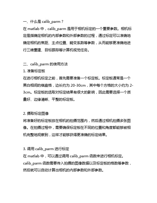
一、什么是calib_parm?在matlab中,calib_parm是用于相机标定的一个重要参数。
相机标定是指确定相机的内部参数和外部参数的过程,通过标定可以准确地确定相机的焦距、主点位置、畸变系数等参数,从而能够更准确地进行三维重建、目标跟踪等计算机视觉任务。
二、calib_parm的使用方法1. 准备标定板在进行相机标定之前,首先需要准备一个标定板。
标定板通常是一个黑白相间的棋盘格,边长约为20-30cm,其中每个方格的大小约为2-3cm。
标定板的选取对标定结果有很大的影响,因此需要选择一个质量好、边缘清晰、平整的标定板。
2. 摄取标定图像将准备好的标定板放在相机的拍摄范围内,然后通过相机拍摄多张图像。
在拍摄过程中,需要确保标定板在不同的位置和角度都能够被相机完整地观察到,这样才能够获得更准确的标定结果。
3. 调用calib_parm进行标定在matlab中,可以通过调用calib_parm函数来进行相机标定。
calib_parm函数需要传入拍摄的图像数据以及标定板的格数等参数,然后就可以自动计算出相机的内部参数和外部参数。
4. 分析标定结果标定完成后,可以通过调用calib_result函数来对标定结果进行分析。
calib_result函数可以输出相机的内部参数矩阵、相机的畸变系数、相机的旋转矩阵和平移向量等参数,这些参数对于后续的计算机视觉任务非常重要。
三、注意事项1. 标定图像的质量对标定结果有很大的影响,因此需要尽量保证拍摄的图像清晰、亮度均匀。
2. 在摄取标定图像时,需要保证标定板在不同位置和角度都能够被完整地观察到,这样才能够获得准确的标定结果。
3. 在调用calib_parm进行标定时,需要正确传入标定板的格数等参数,以确保标定结果的准确性和稳定性。
四、总结通过对calib_parm的使用方法进行了解,可以更加准确地进行相机标定,从而为后续的计算机视觉任务奠定良好的基础。
在实际应用中,需要根据具体的场景和需求来合理选择标定板、调整摄取图像的参数,并且注意事项也需要认真遵守,这样才能够获得准确可靠的标定结果。
matlab相机定标工具箱程序的算法原理
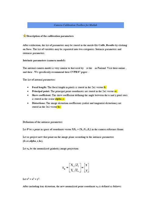
Camera Calibration Toolbox for MatlabDescription of the calibration parametersAfter calibration, the list of parameters may be stored in the matab file Calib_Results by clicking on Save. The list of variables may be separated into two categories: Intrinsic parameters and extrinsic parameters.Intrinsic parameters (camera model):The internal camera model is very similar to that used by at the in Finland. Visit their online , and their . We specifically recommend their CVPR'97 paper: .The list of internal parameters:•Focal length: The focal length in pixels is stored in the 2x1 vector fc.•Principal point: The principal point coordinates are stored in the 2x1 vector cc.•Skew coefficient: The skew coefficient defining the angle between the x and y pixel axes is stored in the scalar alpha_c.•Distortions: The image distortion coefficients (radial and tangential distortions) are stored in the 5x1 vector kc.Definition of the intrinsic parameters:Let P be a point in space of coordinate vector XX c = [X c;Y c;Z c] in the camera reference frame.Let us project now that point on the image plane according to the intrinsic parameters(fc,cc,alpha_c,kc).Let x n be the normalized (pinhole) image projection:Let r2 = x2 + y2.After including lens distortion, the new normalized point coordinate x d is defined as follows:where dx is the tangential distortion vector:Therefore, the 5-vector kc contains both radial and tangential distortion coefficients (observe that the coefficient of 6th order radial distortion term is the fifth entry of the vector kc).It is worth noticing that this distortion model was first introduced by Brown in 1966 and called "Plumb Bob" model (radial polynomial + "thin prism" ). The tangential distortion is due to "decentering", or imperfect centering of the lens components and other manufacturing defects in a compound lens. For more details, refer to Brown's original publications listed in the .Once distortion is applied, the final pixel coordinates x_pixel = [x p;y p] of the projection of P on the image plane is:Therefore, the pixel coordinate vector x_pixel and the normalized (distorted) coordinate vector x d are related to each other through the linear equation:where KK is known as the camera matrix, and defined as follows:In matlab, this matrix is stored in the variable KK after calibration. Observe that fc(1) and fc(2) are the focal distance (a unique value in mm) expressed in units of horizontal and vertical pixels. Both components of the vector fc are usually very similar. The ratio fc(2)/fc(1), often called "aspect ratio", is different from 1 if the pixel in the CCD array are not square. Therefore, the camera model naturally handles non-square pixels. In addition, the coefficient alpha_c encodes the angle between the x and y sensor axes. Consequently, pixels are even allowed to benon-rectangular. Some authors refer to that type of model as "affine distortion" model.In addition to computing estimates for the intrinsic parameters fc, cc, kc and alpha_c, the toolbox also returns estimates of the uncertainties on those parameters. The matlab variables containing those uncertainties are fc_error, cc_error, kc_error, alpha_c_error. For information, those vectors are approximately three times the standard deviations of the errors of estimation.Here is an example of output of the toolbox after optimization:In this case fc = [657.30254 ; 657.74391] and fc_error = [0.28487 ; 0.28937], cc = [302.71656 ; 242.33386], cc_error = [0.59115 ; 0.55710], ...Important Convention: Pixel coordinates are defined such that [0;0] is the center of the upper left pixel of the image. As a result, [nx-1;0] is center of the upper right corner pixel, [0;ny-1] is the center of the lower left corner pixel and [nx-1;ny-1] is the center of the lower right corner pixel where nx and ny are the width and height of the image (for the images of the first example,nx=640 and ny=480). One matlab function provided in the toolbox computes that direct pixel projection map. This function is project_points2.m. This function takes in the 3D coordinates of a set of points in space (in world reference frame or camera reference frame) and the intrinsic camera parameters (fc,cc,kc,alpha_c), and returns the pixel projections of the points on the image plane. See the information given in the function.The inverse mapping:The inverse problem of computing the normalized image projection vector x n from the pixel coordinate x_pixel is very useful in most machine vision applications. However, because of the high degree distortion model, there exists no general algebraic expression for this inverse map (also called normalization). In the toolbox however, a numerical implementation of inverse mapping is provided in the form of a function: normalize.m. Here is the way the function should be called: x n = normalize(x_pixel,fc,cc,kc,alpha_c). In that syntax, x_pixel and x n may consist of more than one point coordinates. For an example of call, see the matlab functioncompute_extrinsic_init.m.Reduced camera models:Currently manufactured cameras do not always justify this very general optical model. For example, it now customary to assume rectangular pixels, and thus assume zero skew (alpha_c=0). It is in fact a default setting of the toolbox (the skew coefficient not being estimated). Furthermore, the very generic (6th order radial + tangential) distortion model is often not considered completely. For standard field of views (non wide-angle cameras), it is often not necessary (and not recommended) to push the radial component of distortion model beyond the 4th order (i.e. keeping kc(5)=0). This is also a default setting of the toolbox. In addition, the tangential component of distortion can often be discarded (justified by the fact that most lenses currently manufactured do not have imperfection in centering). The 4th order symmetric radial distortion with no tangential component (the last three component of kc are set to zero) is actually the distortion model used by . Another very common distortion model for good optical systems or narrow field of view lenses is the second order symmetric radial distortion model. In that model, only the first component of the vector kc is estimated, while the other four are set to zero. This model is also commonly used when a few images are used for calibration (too little data to estimate a more complex model). Aside from distortions and skew, other model reductions are possible. For example, when only a few images are used for calibration (e.g. one, two or three images) the principal point cc is often very difficult to estimate reliably . It is known to be one of the most difficult part of the native perspective projection model to estimate (ignoring lens distortions). If this is the case, it is sometimes better (and recommended) to set the principal point at the center of the image (cc = [(nx-1)/2;(ny-1)/2]) and not estimate it further. Finally, in few rare instances, it may be necessary to reject the aspect ratio fc(2)/fc(1) from the estimation. Although this final model reduction step is possible with the toolbox, it is generally not recommended as the aspect ratio is often 'easy' to estimate very reliably. For more information on how to perform model selection with the toolbox, visit the .Correspondence with Heikkil䧳notation:In the original , the internal parameters appear with slightly different names. The following table gives the correspondence between the two notation schemes:A few comments on Heikkil䧳model:•Skew is not estimated (alpha_c=0). It may not be a problem as most cameras currently manufactured do not have centering imperfections.•The radial component of the distortion model is only up to the 4th order. This is sufficient for most cases.•The four variables (f,Du,Dv,su) replacing the 2x1 focal vector fc are in general impossible to estimate separately. It is only possible if two of those variables are known(for example the metric focal value f and the scale factor su). See for more information.Correspondence with Reg Willson's notation:In his original , uses a different notation for the camera parameters. The following table gives the correspondence between the two notation schemes:Willson uses a first order radial distortion model (with an additional constant kappa1) that does not have an easy closed-form corespondence with our distortion model (encoded with the coefficients kc(1),...,kc(5)). However, we included in the toolbox a function calledwillson_convert that converts the entire set of Willson's parameters into our parameters (including distortion). This function is called in another function willson_read that directly loads in a calibration result file generated by Willson's code and computes the set parameters (intrinsic and extrinsic) following our notation (to use that function, first set the matlab variable calib_file to the name of the original willson calibration file).A few extra comments on Willson's model:•Similarly to Heikkil䧳model, the skew is not included in the model (alpha_c=0).•Similarly to Heikkil䧳model, the four variables (f,sx,dpx,dpy) replacing the 2x1 focal vector fc are in general impossible to estimate separately. It is only possible if two ofthose variables are known (for example the metric focal value f and the scale factor sx).Extrinsic parameters:•Rotations: A set of n_ima 3x3 rotation matrices Rc_1, Rc_2,.., Rc_20 (assuming n_ima=20).•Translations: A set of n_ima 3x1 vectors Tc_1, Tc_2,.., Tc_20 (assuming n_ima=20).Definition of the extrinsic parameters:Consider the calibration grid #i (attached to the i th calibration image), and concentrate on the camera reference frame attahed to that grid.Without loss of generality, take i = 1. The following figure shows the reference frame (O,X,Y,Z) attached to that calibration gid.Let P be a point space of coordinate vector XX = [X;Y;Z] in the grid reference frame (reference frame shown on the previous figure).Let XX c = [X c;Y c;Z c] be the coordinate vector of P in the camera reference frame.Then XX and XX c are related to each other through the following rigid motion equation:XX c = Rc_1 * XX + Tc_1In particular, the translation vector Tc_1 is the coordinate vector of the origin of the grid pattern (O) in the camera reference frame, and the thrid column of the matrix Rc_1 is the surface normal vector of the plane containing the planar grid in the camera reference frame.The same relation holds for the remaining extrinsic parameters (Rc_2,Tc_2), (Rc_3,Tc_3), ... , (Rc_20,Tc_20).Once the coordinates of a point is expressed in the camera reference frame, it may be projected on the image plane using the intrinsic camera parameters.The vectors omc_1, omc_1, ... , omc_20 are the rotation vectors associated to the rotation matrices Rc_1, Rc_1, ... , Rc_20. The two are related through the rodrigues formula. For example, Rc_1 = rodrigues(omc_1).Similarly to the intrinsic parameters, the uncertainties attached to the estimates of the extrinsic parameters omc_i, Tc_i (i=1,...,n_ima) are also computed by the toolbox. Those uncertainties are stored in the vectors omc_error_1,..., omc_error_20, Tc_error_1,..., Tc_error_20 (assuming n_ima = 20) and represent approximately three times the standard deviations of the errors of estimation.。
相机标定方法 matlab

相机标定方法 matlab相机标定是计算机视觉中的重要部分之一,它是通过测量图像上的物体点和其在相机坐标系下对应的点坐标,来估算相机内部参数和外部参数的过程。
相机内部参数通常包括焦距、主点位置和畸变参数等,它们决定了图像中的物体大小和位置。
相机外部参数包括相机的旋转和平移参数,它们决定了物体在相机坐标系下的坐标。
在 MATLAB 中,相机标定是通过图像处理工具箱中的“camera calibration”函数实现的。
在执行相机标定之前,需要准备一组称为标定板的物体,并在不同位置和姿态下拍摄多个图像。
标定板可以是长方形或正方形的棋盘格,也可以是自定义形状的物体,但是必须有已知的三维坐标和相应的二维坐标对。
以下是一个基本的相机标定流程,详细介绍了如何使用 MATLAB 实现相机标定。
1. 准备标定板需要准备一个标定板。
标定板可以是一个黑白棋盘格或自定义形状的物体。
在这里,我们将使用一个 9x7 的黑白棋盘格。
2. 采集标定图像接下来,需要拍摄多个标定图像,并记录标定板在每个图像中的位置和姿态。
对于每个图像,需要至少拍摄 10 张,以确保图像的质量和特征的稳定性。
可以使用不同的相机设置,例如不同的焦距、光圈和曝光时间等,来捕捉标定板的不同姿态。
3. 读取图像和标定板角点在 MATLAB 中,可以使用“imageDatastore”函数读取标定图像并创建一个图像数据存储对象。
接下来,可以使用“detectCheckerboardPoints”函数来检测标定板上的角点。
这个函数会返回一个 Nx2 的矩阵,其中 N 是标定板上检测到的角点数。
4. 定义标定板上角点的空间坐标现在需要定义标定板上角点的空间坐标。
这些坐标可以使用“generateCheckerboardPoints”函数自动生成。
该函数会返回一个 Nx3 的矩阵,其中N 是标定板上的角点数,每一行代表一个角点的空间坐标。
5. 进行相机标定用于相机标定的主要函数是“cameraCalibration”函数。
Matlab图像处理基本操作及摄像机标定

实验三 Matlab图像处理基本操作及摄像机标定(D L T)1、实验目的通过应用Matlab的图像处理基本函数,学习图像处理中的一些基础操作和处理。
理解摄像机标定(DLT)方法的原理,并利用程序实现摄像机内参数和外参数的估计。
2、实验内容1) 读取一幅图像并显示。
2) 检查内存(数组)中的图像。
3) 实现图像直方图均衡化。
4) 读取图像中像素点的坐标值。
5) 保存图像。
6) 检查新生成文件的信息。
7) 使用阈值操作将图像转换为二值图像。
8) 根据RGB图像创建一幅灰度图像。
9) 调节图像的对比度。
10) 在同一个窗口内显示两幅图像。
11) 掌握matlab命令及函数,获取标定块图像的特征点坐标。
12) 根据摄像机标定(DLT)方法原理,编写Matlab程序,估计摄像机内参数和外参数。
3、实验要求:1) 选取一幅图像,根据实验内容1)—10)给出结果。
2) 根据给定的标定块图像及实验内容11),12)进行编程实验。
选取图像:4、实验完成1) 读取一幅图像并显示。
myread=imread('a3.jpg');imshow(myread)2) 检查内存(数组)中的图像。
>> whosName Size Bytes Class Attributes myread 768x1024x3 2359296 uint83) 实现图像直方图均衡化。
myread2=rgb2gray(myread);figure,imhist(myread2)myread3=histeq(myread2);figure,imshow(myread3)01002004) 读取图像中像素点的坐标值。
clcclearimshow('a3.jpg')hold onx_total=[];y_total=[];a=input('ÇëÍõÐÀ²¨ÊäÈëÐèÒª¶ÁÈ¡×ø±êµãµÄ¸öÊý(1~~~100): ')for i=1:a[x,y]=ginput(1);plot(x,y,'+r')text(x+0.5,y+0.5,num2str(i))x_total=[x_total,x];y_total=[y_total,y];enddisp('x=')disp(x_total)disp('y=')disp(y_total)取6个点如下图所示:各点坐标为:x=538.0000 613.0000 682.0000 391.0000 473.5000 266.5000 y=718.2500 656.7500 593.7500 650.7500 487.2500 293.7500 5) 保存图像。
鱼眼相机标定 matlab

鱼眼相机标定 matlab鱼眼相机是一种广角相机,具有大视场角和畸变较大的特点。
在使用鱼眼相机进行图像处理时,必须先进行相机标定,以消除图像畸变,保证图像处理的准确性。
相机标定是指确定相机的内外参数的过程。
内参数是指相机的焦距、像元尺寸等固有参数,而外参数则是相机在世界坐标系下的位姿。
鱼眼相机的标定相对于普通相机而言更加复杂,因为鱼眼相机的畸变较大,无法使用简单的针孔相机模型进行标定。
在 Matlab 中,可以使用 Computer Vision Toolbox 提供的相机标定工具箱进行鱼眼相机标定。
首先,需要准备一组已知的世界坐标系下的特征点和相应的图像坐标系下的特征点。
这些特征点可以是棋盘格的角点或者其他已知的几何形状。
接下来,需要调用 Matlab 中的相机标定函数,通过输入世界坐标系下的特征点和图像坐标系下的特征点,可以得到相机的内外参数。
其中,内参数包括相机的焦距、主点位置等,外参数则包括相机在世界坐标系下的旋转和平移矩阵。
在进行鱼眼相机标定时,需要注意选取合适的标定板和特征点。
由于鱼眼相机的畸变较大,建议选取具有较大畸变的区域进行标定,以提高标定的准确性。
同时,为了获得更好的标定结果,可以使用多组特征点进行标定,并取平均值作为最终的标定结果。
除了使用 Matlab 自带的相机标定工具箱,也可以使用 OpenCV 等其他软件进行鱼眼相机标定。
这些软件提供了更多的标定方法和调试功能,可以根据实际需求进行选择。
在鱼眼相机标定完成后,可以将标定结果应用于图像处理中。
首先,需要对采集到的图像进行畸变校正,即通过标定结果对图像进行去畸变处理。
然后,可以根据相机的内外参数进行尺度恢复、三维重建等图像处理操作。
鱼眼相机标定是使用鱼眼相机进行图像处理的重要步骤。
通过使用Matlab 提供的相机标定工具箱,可以方便地进行鱼眼相机标定,并获得准确的内外参数。
这为后续的图像处理操作提供了可靠的基础。
同时,也可以使用其他软件进行鱼眼相机标定,以满足不同的需求。
Matlab标定工具箱在摄像机定标中的应用
T -T -1
h1 K K h2=0 .
(3)
T -T -1
T -T -1
h1 K K h1=h2 K K h2 .
(4)
收 稿 日 期 :2010-01-07;修 回 日 期 :2010-02-11 作者简介:孙玉青( 1982- ) ,女,山东潍坊人,在读硕士,主要从事图像处理与摄像机定标研究,E- mail:sun_yuqing99@。
和平移向量,
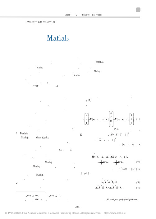
H= h1 h2 h3 λK r1 r2 t ,
r1=
1 λ
K-1h1,
r2=
1 λ
K-1h2
.
(2)
T
根 据 旋 转 矩 阵 的 性 质 , 即 r1 r2=0 和 ‖ rq‖ = ‖r2=1‖ , 每 幅 图 像 可 以 获 得 以 下 两 个 对 摄 像 机 内 参 数矩阵的基本约束,
在图像测量过程以及机器视觉应用中, 常常会 涉及到这样一个概念, 那就是利用摄像机所拍摄到 的图像来还原空间中的物体。 从摄像机获取的图像 信息出发计算三维空间中物体的几何信息, 并由此 重建和识别物体, 而空间物体表面某点的三维几何 位置与其在图像中对应点之间的相互关系是由摄像 机成像的几何模型决定的, 这些几何模型参数就是 摄像机参数。 在大多数条件下这些参数必须通过实 验与计算才能得到, 这一过程被称为摄像机定标[1]。 1 Matlab 简述
本文摄像机定标的基本原理为的平面上其中为模板上点的齐次坐标为模板平面上点投影到图像平面上对应点的齐次坐标分别是摄像机坐标系相对于世界坐标系的旋转矩阵和平移向量每幅图像可以获得以下两个对摄像机内参数矩阵的基本约束atlab标定工具箱在摄像机定标中的应用孙玉青冀小平简述了atlab标定工具箱以及摄像机定标的概念原理和意义给出了摄像机定标中所用的三种坐标系以及它们之间的关系推导出摄像机参数标定算法公式在此基础上利用atlab标定工具箱仿真了棋盘网格的角点标定算法并给出了仿真结果以及误差分析得出了atlab标定工具箱在摄像机定标方面运用的有效性及算法的正关键词
Matlab摄像机标定工具箱的使用说明
摄像机标定工具箱Matlab 摄像机标定工具箱工具箱下载:说明文档:安装:将下载的工具箱文件解压缩,将目录toolbox_calib 拷贝到Matlab 的目录下。
采集图像:采集的图像统一命名后,拷贝到toolbox_calib 目录中。
命名规则为基本名和编号,基本名在前,后面直接跟着数字编号。
编号最多为3位十进制数字。
1.1.1 标定模型内参数标定采用的模型如式(1-1)所示,Brown 畸变模型式(1-2)所示。
⎥⎥⎥⎦⎤⎢⎢⎢⎣⎡=⎥⎥⎥⎦⎤⎢⎢⎢⎣⎡⎥⎥⎥⎦⎤⎢⎢⎢⎣⎡=⎥⎥⎥⎦⎤⎢⎢⎢⎣⎡11//100011100c c in c c c c ys x y x M z y z x v k u k k v u (1-1) 式中:(u , v )是特征点的图像坐标,(x c , y c , z c )是特征点在摄像机坐标系的坐标,k x 、k y 是焦距归一化成像平面上的成像点坐标到图像坐标的放大系数,k s 是对应于图像坐标u 、v 的摄像机的x 、y 轴之间不垂直带来的耦合放大系数,(u 0, v 0)是光轴中心点的图像坐标即主点坐标,(x c 1, y c 1)是焦距归一化成像平面上的成像点坐标。
k s =c k x ,c 是摄像机的实际y 轴与理想y 轴之间的夹角,单位为弧度。
⎪⎩⎪⎨⎧++++++=++++++=1142123654221112124113654221112)2()1()2(2)1(c c c c c c c c c d c c c c c c c c c c d c y x k y r k r k r k r k y y x r k y x k r k r k r k x x (1-2) 式中:(x c 1d , y c 1d )是焦距归一化成像平面上的成像点畸变后的坐标,k c 1是2阶径向畸变系数,k c 2是4阶径向畸变系数,k c 5是6阶径向畸变系数,k c 3、k c 4是切向畸变系数,r 为成像点到摄像机坐标系原点的距离,r 2= x c 12 + y c 12。
原创摄像机标定
1、基于matlab2016的摄像机标定操作流程:(1) 点击matlab2016 界面中APP 菜单下Camera Calibration 图标;(2) 在Camera Calibration 界面当中点击Add Image 图标,加载相机采集的包含激光条纹的靶标图像(在相机标定中激光条纹不参与标定,但它将用于激光传感器的标定),并在输入靶标方格尺寸(小方格长度尺寸),点击确定。
(3) 点击Calibrate 图标,对相机进行标定,点击Export camera Parameter 获取相机部分参数。
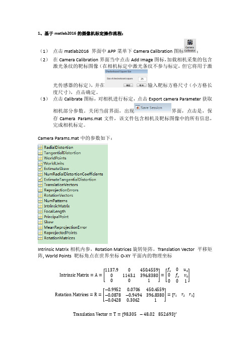
关闭当前界面,出现界面,点击是,保存Camera Params.mat 文件,该文件包含相机及靶标图像中的所有信息,完成相机标定。
Camera Params.mat 中的参数如下:Intrinsic Matrix 相机内参,Rotation Matrices 旋转矩阵,Translation Vector 平移矩阵, World Points 靶标角点在世界坐标O-XY 平面内的物理坐标Intrinsic Matrix =A =[1137.90450.455901143.1396.8380001]=[f x 0u 00f y v 001] Rotation Matrices =R =[−0.99520.0706450.4559−0.0878−0.9494396.8380−0.04280.3062 1]=[r 1r 2r 3]Translation Vector =T =[98.305 −48.02 852.693]′World Points =(X w ,Y w )其中,World Points 靶标角点将参与激光传感器标定中特征点的求解。
像素坐标与世界坐标之间的转换关系:s [uv 1]=A [R T ][X Y Z 1]=[f x 0u o 0f y v o 001][r 1 r 2 r 3 t ][X Y Z 1]2、激光器标定图2-1激光传感器标定模型激光传感器标定就是获取不同位置下的三维特征点,并对其进行平面拟合,获取光平面参数,从图2-1中可以得出如下信息:(1)摄像机标定,获取相机内外参数;(2)激光条纹中心提取,获取激光条纹中心坐标;(3)各坐标系之间的坐标转换。
matlab相机内参数标定原理 -回复

matlab相机内参数标定原理-回复导语:相机内参数标定是摄影测量中的一项重要工作,它通过确定相机的内部参数来提高图像的质量和精度。
本文将介绍相机内参数标定的原理和步骤,以及在Matlab中进行相机标定的具体实现。
一、相机内参数标定的意义和概述(150字)相机内参数是指相机的内部构造和特性,包括焦距、主点位置、像素尺寸、畸变等。
标定相机的内参数可以提高图像的质量和精度,用于计算三维空间中点的坐标。
相机内参数标定是摄影测量的关键步骤之一,对于计算机视觉、机器人导航等应用领域起着重要的作用。
二、相机内参数标定的原理(300字)相机内参数标定的原理是基于针孔成像模型,即相机捕捉到的物体影像是通过相机的中心投影到成像平面上的。
由于相机存在像素尺寸不一致、镜头畸变等问题,所以需要通过标定来确定相机的内参数。
相机内参数标定主要包括焦距、主点位置、径向畸变和切向畸变等参数的确定。
其中,焦距和主点位置确定相机的相对尺度和相对位置,径向畸变参数通过拟合成像圆的畸变效果实现,切向畸变参数通过拟合成像椭圆的畸变效果实现。
标定相机的过程通常需要采集多组不同位置和姿态的标定板图像,并通过标定板上已知的特征点来计算出相机的内参数。
这些特征点通过角点检测算法获取,然后通过最小二乘法拟合得到相机的内参数矩阵。
三、Matlab相机内参数标定的步骤(600字)在Matlab中,可以使用Computer Vision Toolbox提供的函数来实现相机内参数标定。
以下是一步一步的实现过程:1. 准备标定板:选择一个标定板,常见的有棋盘格、圆点标定板等。
确保标定板的特征点能够被准确检测到。
2. 采集标定板图像:在不同位置和姿态下,使用相机采集多组标定板图像。
图像的数量越多,标定结果越准确。
3. 检测标定板角点:使用角点检测算法,如Harris角点检测或亚像素角点检测,来获取标定板图像中的特征点坐标。
4. 优化角点坐标:使用亚像素精确化算法对检测到的角点坐标进行优化,提高标定的精度。
Matlab中利用工具箱进行摄像头标定
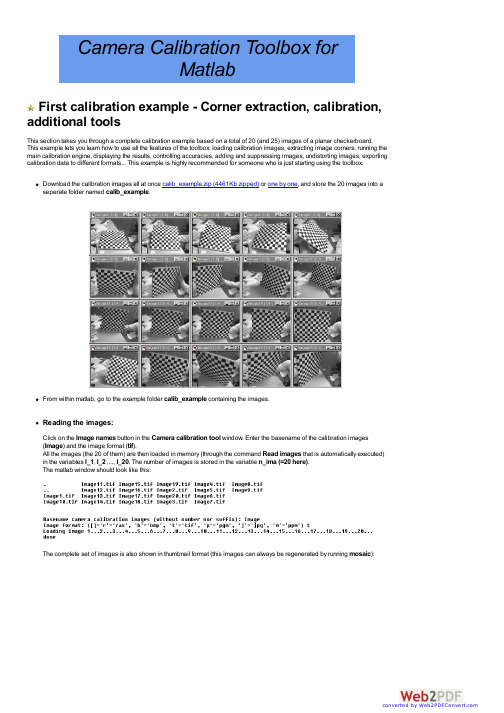
Camera Calibration Toolbox forMatlabFirst calibration example - Corner extraction, calibration, additional toolsThis section takes you through a complete calibration example based on a total of 20 (and 25) images of a planar checkerboard. This example lets you learn how to use all the features of the toolbox: loading calibration images, extracting image corners, running the main calibration engine, displaying the results, controlling accuracies, adding and suppressing images, undistorting images, exporting calibration data to different formats... This example is highly recommended for someone who is just starting using the toolbox.Download the calibration images all at once calib_example.zip (4461Kb zipped) or one by one, and store the 20 images into a seperate folder named calib_example.From within matlab, go to the example folder calib_example containing the images.Reading the images:Click on the Image names button in the Camera calibration tool window. Enter the basename of the calibration images (Image) and the image format (tif).All the images (the 20 of them) are then loaded in memory (through the command Read images that is automatically executed) in the variables I_1, I_2 ,..., I_20. The number of images is stored in the variable n_ima (=20 here).The matlab window should look like this:The complete set of images is also shown in thumbnail format (this images can always be regenerated by running mosaic):If the OUT OF MEMORY error message occurred during image reading, that means that your computer does not have enough RAM to hold the entire set of images in local memory. This can easily happen of you are running the toolbox on a 128MB or less laptop for example. In this case, you can directly switch to the memory efficient version of the toolbox by running calib_gui and selecting the memory efficient mode of operation. The remaining steps of calibration (grid corner extraction and calibration) are exactly the same. Note that in memory efficient mode, the thumbnail image is not displayed since the calibration images are not loaded all at once.Extract the grid corners:Click on the Extract grid corners button in the Camera calibration tool window.Press "enter" (with an empty argument) to select all the images (otherwise, you would enter a list of image indices like [2 5 8 10 12] to extract corners of a subset of images). Then, select the default window size of the corner finder: wintx=winty=5 by pressing "enter" with empty arguments to the wintx and winty question. This leads to a effective window of size 11x11 pixels.The corner extraction engine includes an automatic mechanism for counting the number of squares in the grid. This tool is specially convenient when working with a large number of images since the user does not have to manually enter the number of squares in both x and y directions of the pattern. On some very rare occasions however, this code may not predict the right number of squares. This would typically happen when calibrating lenses with extreme distortions. At this point in the corner extraction procedure, the program gives the option to the user to disable the automatic square counting code. In that special mode, the user would be prompted for the square count for every image. In this present example, it is perfectly appropriate to keep working in the default mode (i.e. with automatic square counting activated), and therefore, simply press "enter" with an empty argument. (NOTE: it is generally recommended to first use the corner extraction code in this default mode, and then, if need be, re-process the few images with "problems")The first calibration image is then shown on Figure 2:Click on the four extreme corners on the rectangular checkerboard pattern. The clicking locations are shown on the four following figures (WARNING: try to click accurately on the four corners, at most 5 pixels away from the corners. Otherwise some of theOrdering rule for clicking: The first clicked point is selected to be associated to the origin point of the reference frame attached to the grid. The other three points of the rectangular grid can be clicked in any order. This first-click rule is especially important if you need to calibrate externally multiple cameras (i.e. compute the relative positions of several cameras in space). When dealing with multiple cameras, the same grid pattern reference frame needs to be consistently selected for the different camera images (i.e. grid points need to correspond across the different camera views). For example, it is a requirement to run the stereo calibration toolbox stereo_gui.m (try help stereo_gui and visit the fifth calibration example page for more information).The boundary of the calibration grid is then shown on Figure 2:Enter the sizes dX and dY in X and Y of each square in the grid (in this case, dX=dY=30mm=default values):Note that you could have just pressed "enter" with an empty argument to select the default values. The program automatically counts the number of squares in both dimensions, and shows the predicted grid corners in absence of distortion:If the predicted corners are close to the real image corners, then the following step may be skipped (if there is not much image distortion). This is the case in that present image: the predicted corners are close enough to the real image corners. Therefore, it is not necessary to "help" the software to detect the image corners by entering a guess for radial distortion coefficient. Press "enter", and the corners are automatically extracted using those positions as initial guess.The image corners are then automatically extracted, and displayed on figure 3 (the blue squares around the corner points show the limits of the corner finder window):The corners are extracted to an accuracy of about 0.1 pixel.Follow the same procedure for the 2nd, 3rd, ... , 14th images. For example, here are the detected corners of image 2, 3, 4, 5, 6 and 7:Observe the square dimensions dX, dY are always kept to their original values (30mm).Sometimes, the predicted corners are not quite close enough to the real image corners to allow for an effective corner extraction. In that case, it is necessary to refine the predicted corners by entering a guess for lens distortion coefficient. This situation occurs at image 15. On that image, the predicted corners are:Observe that some of the predicted corners within the grid are far enough from the real grid corners to result into wrong extractions. The cause: image distortion. In order to help the system make a better guess of the corner locations, the user is free to manually input a guess for the first order lens distortion coefficient kc (to be precise, it is the first entry of the full distortion coefficient vector kc described at this page). In order to input a guess for the lens distortion coefficient, enter a non-empty string to the question Need of an initial guess for distortion? (for example 1). Enter then a distortion coefficient of kc=-0.3 (in practice, this number is typically between -1 and 1).According to this distortion, the new predicted corner locations are:If the new predicted corners are close enough to the real image corners (this is the case here), input any non-empty string (such as 1) to the question Satisfied with distortion?. The subpixel corner locations are then computed using the new predicted locations (with image distortion) as initial guesses:If we had not been satisfied, we would have entered an empty-string to the question Satisfied with distortion? (by directly pressing "enter"), and then tried a new distortion coefficient kc. Y ou may repeat this process as many times as you want until satisfied with the prediction (side note: the values of distortion used at that stage are only used to help corner extraction and will not affect at all the next main calibration step. In other words, these values are neither used as final distortion coefficients, nor used as initial guesses for the true distortion coefficients estimated through the calibration optimization stage).The final detected corners are shown on Figure 3:Repeat the same procedure on the remaining 5 images (16 to 20). On these images however, do not use the predicted distortion option, even if the extracted corners are not quite right. In the next steps, we will correct them (in this example, we could have not used this option for image 15, but that was quite useful for illustration).After corner extraction, the matlab data file calib_data.mat is automatically generated. This file contains all the information gathered throughout the corner extraction stage (image coordinates, corresponding 3D grid coordinates, grid sizes, ...). This file is only created in case of emergency when for example matlab is abruptly terminated before saving. Loading this file would prevent you from having to click again on the images.During your own calibrations, when there is a large amount of distortion in the image, the program may not be able to automatically count the number of squares in the grid. In that case, the number of squares in both X and Y directions have to be entered manually. This should not occur in this present example.Another problem may arise when performing your own calibrations. If the lens distortions are really too severe (for fisheye lenses for example), the simple guiding tool based on a single distortion coefficient kc may not be sufficient to provide good enough initial guesses for the corner locations. For those few difficult cases, a script program is included in the toolbox that allows for a completely manual corner extraction (i.e. one click per corner). The script file is called manual_corner_extraction.m (in memory efficient mode, you should use manual_corner_extraction_no_read.m instead) and should be executed AFTER the traditional corner extaction code (the script relies on data that were computed by the traditional corner extraction code -square count, grid size, order of points, ...- even if the corners themselves were wrongly detected). Obviously, this method for corner extraction could be extremely time consuming when applied on a lot of images. It therefore recommended to use it as a last resort when everything else has failed. Most users should never have to worry about this, and it will not happen in this present calibration example.Main Calibration step:After corner extraction, click on the button Calibration of the Camera calibration tool to run the main camera calibrationprocedure.Calibration is done in two steps: first initialization, and then nonlinear optimization.The initialization step computes a closed-form solution for the calibration parameters based not including any lens distortion (program name: init_calib_param.m).The non-linear optimization step minimizes the total reprojection error (in the least squares sense) over all the calibration parameters (9 DOF for intrinsic: focal, principal point, distortion coefficients, and 6*20 DOF extrinsic => 129 parameters). For a complete description of the calibration parameters, click on that link. The optimization is done by iterative gradient descent with an explicit (closed-form) computation of the Jacobian matrix (program name: go_calib_optim.m).The Calibration parameters are stored in a number of variables. For a complete description of them, visit this page. Notice that the skew coefficient alpha_c and the 6th order radial distortion coefficient (the last entry of kc) have not been estimated (this is the default mode). Therefore, the angle between the x and y pixel axes is 90 degrees. In most practical situations, this is a very good assumption. However, later on, a way of introducing the skew coefficient alpha_c in the optimization will be presented. Observe that only 11 gradient descent iterations are required in order to reach the minimum. This means only 11 evaluations of the reprojection function + Jacobian computation and inversion. The reason for that fast convergence is the quality of the initial guess for the parameters computed by the initialization procedure.For now, ignore the recommendation of the system to reduce the distortion model. The reprojection error is still too large to make a judgement on the complexity of the model. This is mainly because some of the grid corners were not very precisely extracted for a number of images.Click on Reproject on images in the Camera calibration tool to show the reprojections of the grids onto the original images. These projections are computed based on the current intrinsic and extrinsic parameters. Input an empty string (just press "enter") to the question Number(s) of image(s) to show ([] = all images) to indicate that you want to show all the images:The following figures shows the first four images with the detected corners (red crosses) and the reprojected grid corners (circles).The reprojection error is also shown in the form of color-coded crosses:In order to exit the error analysis tool, right-click on anywhere on the figure (you will understand later the use of this option). Click on Show Extrinsic in the Camera calibration tool. The extrinsic parameters (relative positions of the grids with respect to the camera) are then shown in a form of a 3D plot:On this figure, the frame (O c,X c,Y c,Z c) is the camera reference frame. The red pyramid corresponds to the effective field of view of the camera defined by the image plane. T o switch from a "camera-centered" view to a "world-centered" view, just click on the Switch to world-centered view button located at the bottom-left corner of the figure.On this new figure, every camera position and orientation is represented by a green pyramid. Another click on the Switch to camera-centered view button turns the figure back to the "camera-centered" plot.Looking back at the error plot, notice that the reprojection error is very large across a large number of figures. The reason for that is that we have not done a very careful job at extracting the corners on some highly distorted images (a better job could havebeen done by using the predicted distortion option). Nevertheless, we can correct for that now by recomputing the image corners on all images automatically. Here is the way it is going to be done: press on the Recomp. corners button in the main Camera calibration tool and select once again a corner finder window size of wintx = winty = 5 (the default values):T o the question Number(s) of image(s) to process ([] = all images) press "enter" with an empty argument to recompute thecorners on all the images. Enter then the mode of extraction: the automatic mode (auto) uses the re-projected grid as initial guess locations for the corner, the manual mode lets the user extract the corners manually (the traditional corner extraction method). In the present case, the reprojected grid points are very close to the actual image corners. Therefore, we select the automatic mode: press "enter" with an empty string. The corners on all images are then recomputed. your matlab window should look like:Run then another calibration optimization by clicking on Calibration:Observe that only six iterations were necessary for convergence, and no initialization step was performed (the optimization started from the previous calibration result). The two values 0.12668 and 0.12604 are the standard deviation of the reprojection error (in pixel) in both x and y directions respectively. Observe that the uncertainties on the calibration parameters are also estimated. The numerical values are approximately three times the standard deviations.After optimization, click on Save to save the calibration results (intrinsic and extrinsic) in the matlab file Calib_Results.matFor a complete description of the calibration parameters, click on that link.Once again, click on Reproject on images to reproject the grids onto the original calibration images. The four first images looklike:Click on Analyse error to view the new reprojection error (observe that the error is much smaller than before):After right-clicking on the error figure (to exit the error-analysis tool), click on Show Extrinsic to show the new 3D positions of the grids with respect to the camera:A simple click on the Switch to world-centered view button changes the figure to this:The tool Analyse error allows you to inspect which points correspond to large errors. Click on Analyse error and click on the figure region that is shown here (upper-right figure corner):After clicking, the following information appears in the main Matlab window:This means that the corresponding point is on image 18, at the grid coordinate (0,0) in the calibration grid (at the origin of the pattern). The following image shows a close up of that point on the calibration image (before, exit the error inspection tool by clicking on the right mouse button anywhere within the figure):The error inspection tool is very useful in cases where the corners have been badly extracted on one or several images. In such a case, the user can recompute the corners of the specific images using a different window size (larger or smaller).For example, let us recompute the image corners using a window size (wintx=winty=9) for all 20 images except for images 20 (use wintx=winty=5), images 5, 7, 8, 19 (use wintx=winty=7), and images 18 (use wintx=winty=8). The extraction of the corners should be performed with three calls of Recomp. corners. At the first call of Recomp. corners, select wintx=winty=9, choose to process images 1, 2, 3, 4, 6, 9, 10, 11, 12, 13, 14, 15, 16 and 17, and select the automatic mode (the reprojections are already very close to the actual image corners):At the second call of Recomp. corners, select wintx=winty=8, choose to process image 18 and select once again the automatic mode:At the third call of Recomp. corners, select wintx=winty=7, choose to process images 5, 7, 8 and 19 and select once again the automatic mode:Re-calibrate by clicking on Calibration:Observe that the reprojection error (0.11689,0.11500) is slightly smaller than the previous one. In addition, observe that the uncertainties on the calibration parameters are also smaller. Inspect the error by clicking on Analyse error:Let us look at the previous point of interest on image 18, at the grid coordinate (0,0) in the calibration grid. For that, click on Reproject on images and select to show image 18 only (of course, before that, you must exit the error inspection tool by right-cliking within the window):A close view at the point of interest (on image 18) shows a smaller reprojection error:Click once again on Save to save the calibration results (intrinsic and extrinsic) in the matlab file Calib_Results.matObserve that the previous calibration result file was copied under Calib_Results_old0.mat (just in case you want to use it later on).Download now the five additional images Image21.tif, Image22.tif, Image23.tif, Image24.tif and Image25.tif and re-calibrate the camera using the complete set of 25 images without recomputing everything from scratch.After saving the five additional images in the current directory, click on Read images to read the complete new set of images:T o show a thumbnail image of all calibration images, run mosaic (if you are running in memory efficient mode, runmosaic_no_read instead).Click on Extract grid corners to extract the corners on the five new images, with default window sizes wintx=winty=5:And go on with the traditional corner extraction on the five images. Afterwards, run another optimization by clicking on Calibration:Next, recompute the image corners of the four last images using different window sizes. Use wintx=winty=9 for images 22 and 24, use wintx=winty=8 for image 23, and use wintx=winty=6 for image 25. Follow the same procedure as previously presented (three calls of Recomp. corners should be enough). After recomputation, run Calibration once again:Click once again on Save to save the calibration results (intrinsic and extrinsic) in the matlab file Calib_Results.matAs an exercise, recalibrate based on all images, except images 16, 18, 19, 24 and 25 (i.e. calibrate on a new set of 20 images).Click on Add/Suppress images.Enter the list of images to suppress ([16 18 19 24 25]):Click on Calibration to recalibrate:It is up to user to use the function Add/Suppress images to activate or de-activate images. In effect, this function simply updates the binary vector active_images setting zeros to inactive images, and ones to active images.The setup is now back to what it was before supressing 5 images 16, 18, 19, 24 and 25. Let us now run a calibration by including the skew factor alpha_c describing the angle between the x and y pixel axes. For that, set the variable est_alpha to one (at the matlab prompt). As an exercise, let us fit the radial distortion model up to the 6th order (up to now, it was up to the 4th order, with tangential distortion). For that, set the last entry of the vector est_dist to one:Then, run a new calibration by clicking on Calibration:Observe that after optimization, the skew coefficient is very close to zero (alpha_c = 0.00042). This leads to an angle between x and y pixel axes very close to 90 degrees (89.976 degrees). This justifies the previous assumption of rectangular pixels (alpha_c = 0). In addition, notice that the uncertainty on the 6th order radial distortion coefficient is very large (the uncertainty is much larger than the absolute value of the coefficient). In this case, it is preferable to disable its estimation. In this case, set the last entry of est_dist to zero:Then, run calibration once again by clicking on Calibration:Judging the result of calibration satisfactory, let us save the current calibration parameters by clicking on Save:In order to make a decision on the appropriate distortion model to use, it is sometimes very useful to visualize the effect of distortions on the pixel image, and the importance of the radial component versus the tangential component of distortion. For this purpose, run the script visualize_distortions at the matlab prompt (this function is not yet linked to any button in the GUI window). The three following images are then produced:The first figure shows the impact of the complete distortion model (radial + tangential) on each pixel of the image. Each arrow represents the effective displacement of a pixel induced by the lens distortion. Observe that points at the corners of the image are displaced by as much as 25 pixels. The second figure shows the impact of the tangential component of distortion. On this plot, the maximum induced displacement is 0.14 pixel (at the upper left corner of the image). Finally, the third figure shows the impact of the radial component of distortion. This plot is very similar to the full distortion plot, showing the tangential component could very well be discarded in the complete distortion model. On the three figures, the cross indicates the center of the image, and the circle the location of the principal point.Now, just as an exercise (not really recommended in practice), let us run an optimization without the lens distortion model (by enforcing kc = [0;0;0;0;0]) and without aspect ratio (by enforcing both components of fc to be equal). For that, set the binary variables est_dist to [0;0;0;0;0] and est_aspect_ratio to 0 at the matlab prompt:Then, run a new optimization by clicking on Calibration:As expected, the distortion coefficient vector kc is now zero, and both components of the focal vector are equal (fc(1)=fc(2)). In practice, this model for calibration is not recommended: for one thing, it makes little sense to estimate skew without aspectratio. In general, unless required by a specific targeted application, it is recommended to always estimate the aspect ratio in themodel (it is the 'easy part'). Regarding the distortion model, people often run optimization over a subset of the distortioncoefficients. For example, setting est_dist to [1;0;0;0] keeps estimating the first distortion coefficient kc(1) while enforcing the three others to zero. This model is also known as the second order symmetric radial distortion model. It is a very viable model,especially when using low distortion optical systems (expensive lenses), or when only a few images are used for calibration.Another very common distortion model is the 4th order symmetric radial distortion with no tangential component (est_kc = [1;1;0;0]). This model, used by Zhang, is justified by the fact that most lenses currently manufactured do not have imperfection in centering (for more information, visit this page). This model could have very well been used in this present example, recallingfrom the previous three figures that the tangential component of the distortion model is significantly smaller that the radialcomponent.Finally, let us run a calibration rejecting the aspect ratio fc(2)/fc(1), the principal point cc, the distortion coefficients kc, and the skew coefficient alpha_c from the optimization estimation. For that purpose, set the four binary variables , center_optim,est_dist and est_alpha to the following values:Generally, if the principal point is not estimated, the best guess for its location is the center of the image:Then, run a new optimization by clicking on Calibration:Observe that the principal point cc is still at the center of the image after optimization (since center_optim=0).Next, load the old calibration results previously saved in Calib_Results.mat by clicking on Load:Additional functions included in the calibration toolbox:Computation of extrinsic parameters only: Download an additional image of the same calibration grid: Image_ext.tif.Notice that this image was not used in the main calibration procedure. The goal of this exercise is to compute the extrinsic parameters attached to this image given the intrinsic camera parameters previously computed.Click on Comp. Extrinsic in the Camera calibration tool, and successively enter the image name without extension (Image_ext), the image type (tif), and extract the grid corners (following the same procedure as previously presented -remember: the first clicked point is the origin of the pattern reference frame). The extrinsic parameters (3D location of the grid in the camera reference frame) is then computed. The main matlab window should look like:The extrinsic parameters are encoded in the form of a rotation matrix (Rc_ext) and a translation vector (Tc_ext). The rotation vector omc_ext is related to the rotation matrix (Rc_ext) through the Rodrigues formula: Rc_ext = rodrigues(omc_ext).Let us give the exact definition of the extrinsic parameters:Let P be a point space of coordinate vector XX = [X;Y;Z] in the grid reference frame (O,X,Y,Z) shown on the following figure:Let XX c = [X c;Y c;Z c] be the coordinate vector of P in the camera reference frame (O c,X c,Y c,Z c).Then XX and XX c are related to each other through the following rigid motion equation:XX c = Rc_ext * XX + Tc_extIn addition to the rigid motion transformation parameters, the coordinates of the grid points in the grid reference frame are also stored in the matrix X_ext. Observe that the variables Rc_ext, Tc_ext, omc_ext and X_ext are not automatically saved into any matlab file.Undistort images: This function helps you generate the undistorted version of one or multiple images given pre-computed intrinsic camera parameters.As an exercise, let us undistort Image20.tif.Click on Undistort image in the Camera calibration tool.Enter 1 to select an individual image, and successively enter the image name without extension (Image20), the image type (tif). The main matlab window should look like this:The initial image is stored in the matrix I, and displayed in figure 2:The undistorted image is stored in the matrix I2, and displayed in figure 3:。
matlab 标定函数 -回复
matlab 标定函数-回复Matlab是一个功能强大的数值计算软件和编程环境,广泛应用于工程、科学和数学领域。
在计算机视觉领域中,图像的标定是一个重要的任务,用于确定相机的内部参数和外部参数。
Matlab提供了一些内置函数和工具箱,帮助用户完成图像的标定任务。
在本文中,我们将详细介绍Matlab的标定函数及其使用方法。
1. 概述标定是指通过测量相机拍摄的图像中的特征点或已知三维世界点与其在图像中的投影之间的对应关系,来估计相机参数的过程。
相机参数包括内部参数(如焦距、主点坐标、畸变参数等)和外部参数(如旋转矩阵和平移向量)。
Matlab提供的标定函数主要有两个,分别是"calibrateCamera"和"cameraCalibrator"。
2. calibrateCamera函数"calibrateCamera"函数是在Computer Vision Toolbox中提供的一个标定函数。
它使用一组已知的世界坐标点和对应的图像坐标点,来估计相机的内部和外部参数。
函数的基本语法如下:cameraParams =calibrateCamera(imagePoints,worldPoints,imageSize)其中,imagePoints是一个包含每个视图图像中的特征点图像坐标的3D数组。
worldPoints是一个包含每个视图中的对应特征点世界坐标的3D数组。
imageSize是一个包含图像的大小的2D数组。
函数返回一个包含相机参数的结构体cameraParams。
3. cameraCalibrator工具箱"cameraCalibrator"是在Image Processing Toolbox中提供的一个交互式标定工具箱。
它提供了一个直观的图形用户界面(GUI),帮助用户收集和处理标定数据,并估计相机参数。
要使用cameraCalibrator工具箱,可以直接在Matlab命令窗口中输入以下命令:cameraCalibrator然后,将打开一个可视化界面,用户可以在其中加载图像序列并选择特征点。
matlab双目标定注意事项

matlab双目标定注意事项在Matlab中进行双目摄像机标定时,有一些重要的注意事项,以确保标定的准确性和可靠性。
以下是一些建议和注意事项:1. 使用高质量的标定板:选择一个高质量的标定板,它的角点应当清晰可辨认,且板的平整度和稳定性对标定结果有重要影响。
通常,使用棋盘格作为标定板是一种常见的选择。
2. 采用多个角点:在标定图像中使用足够多的角点,这有助于提高标定的准确性。
尽量让标定板填满整个图像。
3. 多角度拍摄:在不同的角度和方向拍摄标定图像,以确保标定结果对摄像机的各种位置和方向变化都具有鲁棒性。
4. 确保图像质量:确保图像的清晰度和对比度足够,避免过曝光或欠曝光的情况。
可采用相机参数进行调整,如曝光时间、光圈等。
5. 使用相同的标定板:在进行双目摄像机标定时,确保两个相机使用相同的标定板。
这是因为两个相机的标定板在三维空间中应当有一一对应的关系。
6. 采用相同的相机设置:在标定过程中,确保两个相机使用相同的设置,如焦距、光圈、曝光时间等。
7. 校准相机内参:在进行标定之前,最好先对每个相机进行单独的内参标定,以确保相机参数的准确性。
Matlab提供了`cameraParameters`对象,可以用于保存相机内参。
8. 使用Matlab的`stereoCameraCalibrator`工具箱:Matlab提供了用于双目相机标定的工具箱,其中包括`stereoCameraCalibrator`应用程序。
这个工具可以帮助你在一个交互式环境中进行标定,提供了图形界面来查看标定结果和误差等信息。
9. 考虑径向和切向畸变:标定时考虑畸变参数,特别是径向畸变和切向畸变。
在Matlab 中,可以通过`cameraParameters`对象来存储这些畸变参数。
10. 检查标定结果:在标定完成后,仔细检查标定结果,查看重投影误差等指标,确保标定的准确性。
以上建议和注意事项应当帮助你更好地进行Matlab中的双目摄像机标定。
鱼眼相机标定 matlab

鱼眼相机标定 matlab鱼眼相机是一种广泛应用于计算机视觉领域的特殊相机。
它的镜头呈现出鱼眼的形状,可以捕捉到更广阔的视野。
然而,由于鱼眼相机的镜头特殊性质,其图像会产生畸变,这就需要进行标定来修正这些畸变。
在计算机视觉领域,相机标定是一个重要的任务,它是对相机内部和外部参数进行估计的过程。
相机内部参数包括焦距、主点位置等,而外部参数包括相机的位置和朝向。
相机标定的目的是为了能够准确地将图像中的点对应到世界坐标系中的点,从而实现图像与现实世界的对应关系。
对于鱼眼相机的标定,一般会使用鱼眼相机模型来描述它的畸变特性。
鱼眼相机模型是一种非线性模型,通过对鱼眼图像中的畸变进行建模,可以将畸变校正到一定程度。
鱼眼相机模型有多种形式,常用的包括全视角模型、等距模型和正切模型等。
在Matlab中,可以使用相机标定工具箱来进行鱼眼相机的标定。
该工具箱提供了一系列函数,可以方便地进行相机标定的各个步骤。
首先,需要采集一组具有已知三维坐标的图像,这些图像可以是由标定板或者其他已知几何形状的物体拍摄得到的。
然后,通过使用相机标定工具箱提供的函数,可以对这些图像进行处理,从而得到相机的内部和外部参数。
在标定过程中,首先需要对图像进行去畸变处理。
通过使用鱼眼相机模型,可以将图像中的畸变进行校正,从而得到畸变较小的图像。
然后,可以使用标定板上的已知三维坐标和对应的图像坐标,利用相机标定算法估计相机的内部和外部参数。
最后,可以通过对标定结果进行评估,以确定标定的准确性和可靠性。
相机标定的结果可以用于多个应用领域。
例如,在计算机视觉中,相机标定是进行三维重建、目标检测和跟踪等任务的基础。
在增强现实和虚拟现实领域,相机标定可以用于将虚拟对象与现实世界进行对齐。
此外,在机器人视觉中,相机标定可以用于导航和场景理解等任务。
鱼眼相机标定是计算机视觉领域中的重要任务之一。
通过对鱼眼相机进行标定,可以修正图像中的畸变,从而提高图像的质量和准确性。
三点标定法 matlab

三点标定法 matlab三点标定法是一种在计算机视觉中常用的相机标定技术,通过采集至少三个不同位置的已知空间点在图像上的投影位置来对相机的内参和外参进行估计。
在Matlab中,可以使用Camera Calibration Toolbox来进行三点标定。
以下是使用Matlab进行三点标定的示例代码:1. 准备图像和已知空间点的数据:```matlab% 所有图像数据保存在一个文件夹中imagesFolder = 'image_folder';imageFiles = dir(fullfile(imagesFolder, '*.jpg'));% 已知空间点的3D坐标worldPoints = [0, 0, 0; 0, 100, 0; 100, 100, 0];```2. 遍历图像文件,对每个图像进行处理:```matlabfor i = 1:length(imageFiles)% 读取图像image = imread(fullfile(imagesFolder, imageFiles(i).name));% 检测图像中的特征点imagePoints = detectCheckerboardPoints(image);% 进行标定[cameraParams, estimationErrors] = estimateCameraParameters(imagePoints, worldPoints);% 显示标定结果figure;showExtrinsics(cameraParams, 'PatternCentric');end```这段代码使用了`detectCheckerboardPoints`函数来检测图像中的棋盘格角点,并使用`estimateCameraParameters`函数来进行标定。
最后使用`showExtrinsics`函数显示标定结果。
基于Matlab工具箱的摄像机标定_
Camera Calibration Based on Matlab Toolbox
WANG Jianqiang, ZHANG Haihua ( College of Engineering,Zhejiang Normal University,Jinhua 321004 ,China) Abstract : The camera calibration is an effective way to improve the precision of measuring system. A 2D planar target is introduced to simplify the complicated target for calibration. The intrinsic and extrinsic parameters of the CCD camera are calibrated by the Matlab toolbox. The position relation between two CCD cameras is gained by stereocalibration. Finally ,a model consisted of four steps with a neighboring height of 1. 00mm and an inclined plane was also measured. The measured average height between neighboring steps is 0. 99mm. Key words: machine vision; stereovision measuring system; camera calibration
38
实
matlabcalibrationtoolbox--matlab标定工具的使用方法--去畸。。。

matlabcalibrationtoolbox--matlab标定⼯具的使⽤⽅法--去畸。
2015-04-06 22:45 5407⼈阅读 (2)分类:机器视觉(12)⼀、对于单⽬标定。
1、也就是单个相机的标定,⾸先是⽤⼀个相机拍摄标定板获得⼀定数量的标定板照⽚。
或者下载的⼀定数量的照⽚。
如下:上图CMOS0是相机1拍摄的图⽚序列,CMOS1是相机2拍摄的图⽚序列。
2、将下载的toolbox⽂件解压到⼀个⽬录下,⽀持5.x--8.x版本的matlab。
然后打开matlab软件:file—>SetPath出现如下界⾯。
Add Folder添加toolbox所在的路径。
3、添加好后,就可以在MATLAB的命令栏中输⼊calib_gui 或者calib,回车,运⾏标定程序。
回车后出现如下界⾯:4、选择图⽚进⾏⾓点检测。
选择第⼀项“Standard(all the images are stored in memory)”,出现如下界⾯:此时要保证“Current Directory”为图⽚所在的⽬录:点击“Image Names”按钮。
Command⾏⾥就会将此⽬录下所有的照⽚名字读出来,如下:“Basename camera calibration images (without number nor suffix):”后⾯输⼊:CMOS0_。
出现如下提⽰:“Image format: ([]='r'='ras', 'b'='bmp', 't'='tif', 'p'='pgm','j'='jpg', 'm'='ppm')”后⾯输⼊:b。
matlab就将加载所有符合条件的图⽚。
之后就是检测⾓点,点击第三项:“Extract grid corners ”:回车,选择所有照⽚。
matlab摄像机标定实验报告

摄像机标定实验报告一、实验任务使用工业摄像机拍摄9张标定图片,利用matlab中Camera Calibration Toolbox对摄像机进行标定。
二、实验原理针孔摄像机模型图1 摄像机针孔模型成像摄像机采集图像原理如图1。
物体上发出的光线投射到图像平面,仿佛所有的光线都经过针孔平面上的针孔点,垂直于针孔平面过针孔点的直线为光轴,从针孔到图像平面的距离就是焦距,在图中,摄像机焦距f,物体到摄像机的距离为Z,物体长S,物体在图像上的长度为s。
物体光线、光轴与物体之间组成相似三角形,得到这样的关系−s/f=S/Z。
图2 针孔模型图像平面一针孔点为中心旋转180°把图像平面以针孔点为中心旋转180°。
物体和图像在针孔平面的一边,仿佛所有光线从物体走到图像平面成像的对应点,最后汇集到一点,这个点定义为投影中心[33]。
图3-22中点O为投影中心。
在抽象的针孔模型中点P(X w,Y w,Z w)由通过投影中心O的光线投影到图像平面上,相应的图像点为p(x,y,f)。
成像芯片的中心通常不在光轴上,定义图像平面与光轴交点为主点o c坐标(c x,c y)。
f为透镜的物理焦距,定义f x为焦距长度与像素x轴方向长度的比,定义f y 为焦距长度与像素y轴方向长度的比。
可以得到x=f x(X wZ w)+c x(1)y=f y(Y wZ w)+c y(2)将坐标为(X,Y,Z)的物理点映射到投影平面上坐标为(x,y)的过程叫投影变换。
齐次坐标可以建立这种变换。
齐次坐标把维数为n投影空间的点表示成(n+1)维向量。
图像平面为二维投影空间,可用三维向量表示该平面上的点。
将摄像机参数f x、f y、c x、c y重新排列为一个3×3的矩阵,如M,该矩阵就是摄像机内部参数矩阵。
将物理世界中的点投射到摄像机上,用下式表示:p=MP,其中p=[x yw ],M=[f x0c x0f y c y001],P=[X wY wZ w](3)标定过程摄像机参数f x、f y、c x、c y、倾斜系数需要通过计算得到,这一过程为摄像机标定。
- 1、下载文档前请自行甄别文档内容的完整性,平台不提供额外的编辑、内容补充、找答案等附加服务。
- 2、"仅部分预览"的文档,不可在线预览部分如存在完整性等问题,可反馈申请退款(可完整预览的文档不适用该条件!)。
- 3、如文档侵犯您的权益,请联系客服反馈,我们会尽快为您处理(人工客服工作时间:9:00-18:30)。
摄像机标定工具箱1.1 Matlab 摄像机标定工具箱工具箱下载:/bouguetj/calib_doc/download/index.html说明文档:/bouguetj/calib_doc/安装:将下载的工具箱文件toolbox_calib.zip 解压缩,将目录toolbox_calib 拷贝到Matlab 的目录下。
采集图像:采集的图像统一命名后,拷贝到toolbox_calib 目录中。
命名规则为基本名和编号,基本名在前,后面直接跟着数字编号。
编号最多为3位十进制数字。
1.1.1 标定模型内参数标定采用的模型如式(1-1)所示,Brown 畸变模型式(1-2)所示。
⎥⎥⎥⎦⎤⎢⎢⎢⎣⎡=⎥⎥⎥⎦⎤⎢⎢⎢⎣⎡⎥⎥⎥⎦⎤⎢⎢⎢⎣⎡=⎥⎥⎥⎦⎤⎢⎢⎢⎣⎡11//100011100c c in c c c c ys x y x M z y z x v k u k k v u (1-1) 式中:(u , v )是特征点的图像坐标,(x c , y c , z c )是特征点在摄像机坐标系的坐标,k x 、k y 是焦距归一化成像平面上的成像点坐标到图像坐标的放大系数,k s 是对应于图像坐标u 、v 的摄像机的x 、y 轴之间不垂直带来的耦合放大系数,(u 0, v 0)是光轴中心点的图像坐标即主点坐标,(x c 1, y c 1)是焦距归一化成像平面上的成像点坐标。
k s =αc k x ,αc 是摄像机的实际y 轴与理想y 轴之间的夹角,单位为弧度。
⎪⎩⎪⎨⎧++++++=++++++=1142123654221112124113654221112)2()1()2(2)1(c c c c c c c c c d c c c c c c c c c c d c y x k y r k r k r k r k y y x r k y x k r k r k r k x x (1-2) 式中:(x c 1d , y c 1d )是焦距归一化成像平面上的成像点畸变后的坐标,k c 1是2阶径向畸变系数,k c 2是4阶径向畸变系数,k c 5是6阶径向畸变系数,k c 3、k c 4是切向畸变系数,r 为成像点到摄像机坐标系原点的距离,r 2= x c 12 + y c 12。
1.1.2 操作界面将Matlab 的当前目录设定为含有标定工具箱的目录,即toolbox_calib 目录。
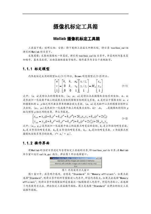
在Matlab 命令窗口运行calib_gui 指令,弹出图1所示选择窗口。
图1 内存使用方式窗口图1窗口中,具有两个选项,分别是“Standard ”和“Memory efficient ”。
如果点击选择“Standard ”,则将目录中的所有图像读入内存中,所需内存较大。
如果点击选择“Memory efficient ”,则将目录中的图像按照需要每次一幅图像读入内存中,所需内存较小。
在选择了内存使用方式后,弹出标定工具箱操作面板。
图2是选择“Standard”后弹出的标定工具箱操作面板。
图2 标定工具箱操作面板图2所示的标定工具箱操作面板具有16个操作命令键,其功能如下:(1) “Image names”键:指定图像的基本名(Basename)和图像格式,并将相应的图像读入内存。
(2) “Read names”键:将指定基本名和格式的图像读入内存。
(3) “Extract grid corners”键:提取网格角点。
(4) “Calibration”键:内参数标定。
(5) “Show Extrinsic”键:以图形方式显示摄像机与标定靶标之间的关系。
(6) “Project on images”键:按照摄像机的内参数以及摄像机的外参数(即靶标坐标系相对于摄像机坐标系的变换关系),根据网格点的笛卡尔空间坐标,将网格角点反投影到图像空间。
(7) “Analyse error”键:图像空间的误差分析(8) “Recomp. corners”键:重新提取网格角点。
(9) “Add/Suppress images”键:增加/删除图像。
(10) “Save”键:保存标定结果。
将内参数标定结果以及摄像机与靶标之间的外参数保存为m文件Calib_results.m,存放于toolbox_calib目录中。
(11) “Load”键:读入标定结果。
从存放于toolbox_calib目录中的标定结果文件Calib_results.mat读入。
(12) “Exit”键:退出标定。
(13) “Comp. Extrinsic”键:计算外参数。
(14) “Undistort image”键:生成消除畸变后的图像并保存。
(15) “Export calib data”键:输出标定数据。
分别以靶标坐标系中的平面坐标和图像中的图像坐标,将每一幅靶标图像的角点保存为两个tex文件。
(16) “Show calib results”键:显示标定结果。
1.1.3 内参数标定预先将命名为Image1~Image20的tif格式的20幅靶标图像保存在toolbox_calib目录中。
当然,采集的靶标图像也可以采用不同的格式,如bmp格式、jpg格式等。
但应注意,用于标定的靶标图像需要采用相同的图像格式。
摄像机的内参数标定过程,如下所述。
(1) 指定图像基本名与图像格式在图2所示的标定工具箱操作面板点击“Image names”键,在Matlab命令窗口分别输入基本名Image和图像格式t,出现下述对话内容:Basename camera calibration images (without number nor suffix): ImageImage format: ([]='r'='ras', 'b'='bmp', 't'='tif', 'p'='pgm', 'j'='jpg', 'm'='ppm') tLoading image 1...2...3...4...5...6...7...8...9...10...11...12...13...14...15...16...17...18...19...20...done同时,在Matlab的图形窗口显示出20幅靶标图像,如图3所示。
Calibration images图3 靶标图像(2) 提取角点在图2所示的标定工具箱操作面板点击“Extract grid corners”键。
⏹在Matlab命令窗口出现“Number(s) of image(s) to process ([] = all images) =”时,输入要进行角点提取的靶标图像的编号并回车。
直接回车表示选用缺省值。
选择缺省值式,对读入的所有的靶标图像进行角点提取。
⏹在Matlab命令窗口出现“Window size for corner finder (wintx and winty): ”时,分别在“wintx ([] = 5) =”和“winty ([] = 5) =”输入行中输入角点提取区域的窗口半宽m和半高n。
m和n为正整数,单位为像素,缺省值为5个像素。
选定m和n后,命令窗口显示角点提取区域的窗口尺寸(2n+1)x(2m+1)。
例如,选择缺省时角点提取区域的窗口尺寸为11x11像素。
⏹在Matlab命令窗口出现“Do you want to use the automatic square counting mechanism(0=[]=default) or do you always want to enter the number of squares manually(1,other)? ”时,选择缺省值0表示自动计算棋盘格靶标选定区域内的方格行数和列数,选择值1表示人工计算并输入棋盘格靶标选定区域内的方格行数和列数。
⏹到显示所选择靶标图像的图形窗口,利用鼠标点击设定棋盘格靶标的选定区域。
点击的第一个角点作为靶标坐标系的原点,顺序点击4个角点形成四边形。
注意,所形成的四边形的边应与棋盘格靶标的网格线基本平行。
否则,影响角点提取精度,甚至导致角点提取错误。
⏹在Matlab命令窗口出现“Size dX of each square along the X direction ([]=100mm) = ”和“Size dY of each square along the Y direction ([]=100mm) = ”时,分别输入方格长度和宽度,单位为mm。
方格长度和宽度的缺省值均为100mm。
⏹在Matlab命令窗口出现“Need of an initial guess for distortion? ([]=no, other=yes) ”时,如果选择no则不输入畸变初始值,如果选择yes则输入畸变初始值。
输入的畸变初始值,将同时赋值给需要估计的5个畸变系数,即径向畸变系数kc(1)、kc(2)、kc(5)和切向畸变系数kc(3)、kc(4)。
如果不估计6阶径向畸变系数kc(5),则kc(5)被赋值为0。
按照上述步骤,对用于标定的每一幅靶标图像进行角点提取。
例如,m=5,n=5时,角点提取区域的窗口尺寸为11x11像素,未输入畸变初始值,此时图像Image6的角点提取结果如图4所示。
图4(a)只标出了待提取角点的位置,图4(b)标出了角点提取区域窗口和提取出的角点。
从图4中可以发现,图4(a)中的十字标记位置与角点具有明显偏差,但在角点附近;图4(b)中的每个角点提取区域窗口包含了角点,表示角点提取结果的十字标记位置与角点位置具有很好的吻合度。
同样在m =5,n =5时,未输入畸变初始值,但通过鼠标点击设定棋盘格靶标的选定区域时,所形成的四边形的边与棋盘格靶标的网格线成较大夹角,此时图像Image1的角点提取结果如图5所示。
从图5中可以发现,图5(a)中的十字标记位置与角点具有明显偏差,部分十字标记远离角点;图5(b)中的很多角点提取区域窗口没有包含角点,表示角点提取结果的十字标记位置并不在角点位置,说明角点提取存在错误。
X Y O The red crosses should be close to the image corners10020030040050060050100150200250300350400450(a)O dX dY X c (in camera frame)Y c (i n c a m e r a f r a m e )Extracted corners10020030040050060050100150200250300350400450(b)图4 合适的靶标选定区域与角点提取结果,(a) 靶标选定区域,(b) 角点提取结果(3) 内参数标定对用于标定的每一幅靶标图像进行角点提取后,在图2所示的标定工具箱操作面板点击“Calibration ”键,即可完成摄像机的内参数标定。