SIMULATION OF IMPERFECT INFORMATION IN VULNERABILITY MODELING FOR INFRASTRUCTURE FACILITIES

合集下载

Knowledge Centred Simulation In Emergency Management Training Systems

Knowledge Centred SimulationInEmergency Management Training SystemsRego GranlundDept. of Computer and Information ScienceLinköping UniversityS-581 83 Linköping, Swedenhttp://www.ida.liu.se/~reggrE-mail: reggr@ida.liu.sewww-version: 1.002-Nov-1995AbstractThis paper describes the research, starting points, problems, and goals, for an on going project in which we are study the design and construction of computer simulation in decision training systems. In particular we are interested in the development of simulation systems for training of staff in emergency decision making and crisis management. The main problem that we are study is how to integrate pedagogical goals into the simulation models in a decision training system for complex dynamic systems.Key words : simulation, micro-world, emergency management, situated learning, situational awareness, autonomous agents1IntroductionThe Problem, Decision Training.2Emergency ManagementEmergency Management, Complex Dynamic Systems,Distributed Decision Making, Natural Decision Making.3Emergency Management TrainingEmergency Management Training, Simulation Problems,Training Organisation.4Research GoalResearch Goal, Research Method, Contributions.5The Micro-World C3FireC3Fire, Requirements met by C3Fire.1 IntroductionThis project deals with design and construction of computer simulation in decision training systems. In particular, with the development of simulation systems for training of commanders and staff in emergency decision making and crisis management. The main problem that we are study is the problem of how to integrate pedagogical goals into the simulation models in a decision training system for complex dynamic systems.The work has been carried out in a research group which focuses on the development and use of knowledge-based systems in real-life applications. This knowledge view is a base for our investigation, and its means that the work focuses on the problem of handling qualitative knowledge in simulated training environments. The project aims at providing design method ideas in form of important properties of training simulation system and of typical modelling difficulties.The ProblemA common design strategy for simulations in training systems, is today often based on a strategy where an object oriented definition of the world is made from a physical model of the world. This strategy can be good if we want to do a simple simulation of the world. But if we want to use the simulation in a training situation, we often want to let pedagogical goals and wanted training situations, influence the simulation. This means that when we define the models and the implementation of the system we must know how the pedagogical goals influence the objects and the events that exist in the simulation. What we do not want to get is a modelling technique that focuses on quantitative data about the physical aspects of the world. We want to have a modelling technique that focuses on the qualitative knowledge about the concepts, the relation between the concepts in the training situation, and on the pedagogical goals of the training. I will refer to this type of simulation as knowledge centred simulation.With knowledge centred simulation we mean that the simulation should change its behaviour depending on the training goals and the knowledge of the students. This is a new and important philosophy when we want to create a simulation system.Decision TrainingSocial systems, like emergency management systems (as forest fire fighting) and military systems, can be characterised by their dynamic behaviour created by co-operating actors. To achieve good performance in these systems, it is important that the people who command and control the system have good understanding of the system and their role in the system. This means that the commanders and staff need to be trained in real-world situations, so they can experience the dynamic behaviour of the system. In these kinds of systems it is often too expensive or humanly impossible to practise in real life situations. In these cases we need training systems where we can train commanders and staff in commanding and controlling a complex system.The goal of a training system for commanders and staff is that they in some way should experience the work situation that they will meet in a real situation. Typical things that they would experience in these kind of training systems are;• How the organisation and the world behave in different kind of common and critical situations.• How the distributed decision making influence their work.• How their work will change with different work-load situation.Important questions and problems for a training system as this is to define pedagogical training goals, and how to generate the world simulation that is needed for these pedagogical training goals.2 Emergency ManagementEmergency management system (as forest fire-fighting etc.), and military systems, can be defined as social systems, in which the decision makers goals are to define and organise a set of co-ordinate actions to reach a goal state and limit the negative consequences on the human, material and economicThe Staff: The commander's task in a staff is to command and control the emergency organisation. This means that they should collect information from the subordinates so that they get a situation awareness. Based on that they should plan and transmit orders to their subordinates, in order to direct and co-ordinate actions between the subordinate units. The staff is decision makers only and do not operate directly on the target system. (Artman 95) describe some of the staff’s work as, gather and sort out relevant and consistent information, make hypothesis about the system, plan one or several appropriate strategies, distribute work and resources to the subordinate units and co-ordinate actions between different units.The Emergency Organisation: In an emergency organisation, the staff’s subordinates are the staff’s tool in their task of controlling the target system. Examples of a subordinate unit can be, a fire fighting unit, an ambulance unit, or a military unit. In large hierarchical organisations as a military brigade, the organisation consist of several levels, companies, platoons, etc. The whole emergency organisation is only semi-controlled by the staff, and can as the target system be viewed as a complex dynamic system.Complex Dynamic SystemThe complexity, and the dynamic and autonomous behaviour of the target-system and the emergency organisation, makes them hard to predict and control. The characteristics of these systems are that the control has to occur in real-time and it is difficult to provide a complete current state of the system because the dynamics of and the relations within the system are not visible. The difficulties in understanding the current state of the system, situation awareness, is an important problem and an important task to train. (Brehmer 94) has defined a complex dynamic system by the following criteria:1. Complexity• It exists a set of disjunctive goals in the system.• It exists a set of related processes in the system.2. Dynamics• The states of the system are changed both autonomously and as a function of the actions that the decision maker makes.• The decision makers have a limited time to make their decisions.3. Opaqueness (not transparency)• Difficult to see the current state of the system.• Difficult to see what relations that exists in the system.Distributed Decision MakingThe decision making in an emergency organisation and in military systems has by (Brehmer 95) been classified as distributed decision making or team decision making. This means that the decision making or the cognition is distributed among the actors in the organisation. The system is also often based on a hierarchical organisation, where the decision makers work in different time scales. The people in the staff work in a higher time level that the subordinate decision makers, and are responsible for the strategic decisions. The problem of distributed decision making makes it important to train communication, and understanding of shared frameworks and goals. Team decision making is distributed decision making where the co-operating actors have different roles, tasks, and items of information in the decision process (Kline & Thordsen 1989; Orasanu & Salas 1993).Natural Decision MakingThe decision made by the staff can be classified as natural decision making. The decision making is not a task. The staff does not set out to ‘make a decision’, they set out to control their resources in a good way. Obtaining this goal requires making many decisions, but decision making is part of a larger activity, not an end in itself. Basic steps in naturalistic decision making are situation assessment and selection of a course of actions. According to (Lipshitz xx), the decision maker does a situation assessment where he or she size up the situation to a situation picture, based on that he or she makes diagnoses, hypotheses and decides a course of action. We can say that the decision maker reacts on the input information and processes it in a context of his or her own expertise. He or she is often not aware of any complex analytic thinking. One interesting decision model is the Recognition-Primed Decisions (RPD) model by (Klein 93). The RPD model is generated from several years of studying command and control performance, and it asserts that people use situation assessment to generate a plausible course of action and use mental simulation to evaluate that course of action.3 Emergency Management TrainingThe thing that is hard to understand or get a good feeling for, by reading a book, is the dynamic behaviour that exists in a complex dynamic system. The dynamic behaviour can be viewed as a behaviour pattern of the target system or the emergency organisation, and should be learned by experience how it is to work as commander for the system. In these cases we can use emergency management training systems to bridge the gap between the theoretical studies and the work situations in the real world. Common training goals for the staff in an emergency management training are; Their task: Understand the work procedures, understanding the current situation, ‘situation awareness’, identifying future critical situations, etc.Distributed Decision:Experience how to exchange information with other persons in the organisation, the others persons needs and goals, and the importance of shared frameworks and goals. Dynamic Behaviour: Experience the dynamic behaviour of the organisation and the target system. Work Situation: Experience time pressure, high information load, inconsistent / missing information. There exist two important problems with this type of training, simulation of the surrounding world, and pedagogical control of the training sessions.Simulation problemsThe simulation of the surrounding world should be is so realistic that it generates the same behaviour pattern ‘gestalts’ as the real world. The demands on the behaviour pattern gestalts are not so important for things that are not with in the training goals, but is very important for the behaviour that is connected to the training goals (Gestrelius 93). The main problem with the simulation is that the real-world systems often are based on co-operating actors. The basic problems are:Naturally Language Interaction: The interaction between the staff and the co-operating actors in the emergency organisation should be in natural language. A common way to solve this is to simplify and restrict the communication, or to use people that make a role-play of the actors in the environment. Activity Simulation: One important goal with the activity simulation is that the combination of all activities should generate the dynamic behaviour of the system. This means that it is hard to simplify a computer simulation and it is also hard for a role-playing person to simulate a number of activities. Training Session Control:The simulation should be controlled by the pedagogical goals. The simulation should change depending on the training goals, the students activity and knowledge. Training OrganisationTraining assistants:Their task is to make a realistic role-play of the humans that exist in the simulation. Their main task is to follow the pedagogical goals, communicate with the staff, react on the commands from the staff and on the information they get from the computer simulation. The main problem for the training assistant is to keep all the processes in the mind and not forget some important response from these activities. Besides the risk that the training assistant becomes overloaded, it is important that the training assistance have good experience and understanding of the pedagogical goals. One large problem for the training assistants is to co-ordinate and synchronise theirs activity so that wanted training situations generates.Training manager: The training manager should follow the activity of staff and direct the session so that it generates a proper training for the staff.Computer Simulation:The computer simulation should be used to support the training assistants with simulation of physical things. In more advanced simulations the computer can have models of human activities so that it can simulate human controlled activities. The simulation should follow the pedagogical goals and react on the students knowledge.The teaching strategies in this type of system use to be base on, briefing and debriefing.4 Research GoalThe problem in focus is to see how we can support the training assistants with a computer simulation tool that simulates some of the activity simulations that the training assistants are responsible for. The main task is to examine the properties of the simulation-tool they may need, and how pedagogical goals can be integrated in to these simulations.Research goalThe problem domain described above is the ground for this work. Based on this problem domain we have a specific research question, that is:• How will the pedagogy in situated learning theories influence the design of computer simulation in decision training systems?The aim of the work is to provide some answers to the question, based on our own interpretation of a literature study in the area, on a study of existing systems and on first-hand experience collected from previous projects and on design, implementation and evaluation of C3Fire, a decision training system. The aim is to bridge the gap between educational theories, dynamic systems theories and computer simulations. The contributions should be more on the methodological rather than on the technical level. The implementation techniques will not be used for improving those techniques in them selves. The goal is to show how these techniques can be used to produce better systems, in the pedagogical point of view. The long time research goal in this research is to define case tools, that supports some methodology to design simulations in emergency management decision training systems.Research MethodResults from a study of existing training systems (Granlund 94ab), indicated that it should be a hard task to create an experimental simulation system. In these training systems, the surrounding world were to complex and the training goals were too unspecified, to be a good research task. On the basis of this we have selected to do an experimental simulation system in a micro-world. A micro-world means that we select some important properties from the real system and create a small and well-controlled environment for our experimentation. The goal of the micro-world system is that we want to have an experimentation platform where we can change different control strategies and study the performance of these. The performance could in this environment be empirically studied by doing different training sessions, where we can compare the trained peoples performance.The environment gives an ability to:• Investigate and train people in commanding and controlling a dynamic system.• Create a knowledge centred training environment.• Create a control structure so that we can produce pedagogical training sessions.• Train people in solving problems in a dynamic environment.ContributionsThe main contributions are:• C3Fire, an environment for investigation and training experimentation of distributed cognition and situational awareness. C3Fire is a, command, control and communication, experimental simulation environment. The system consists of a micro-world that can be used to demonstrate how a training system for forest fire extinguish commanders can be archived.• A discussion of the design, construction and evaluation of the C3Fire environment. The evaluation discussion is based on an experiment series, containing 15 * 4 hours experimentation, with 4 co-operating persons in the micro-world. The goal of the discussion is to give some guidelines that aim towards some methodologies for design and construct decision training systems.It might be worth pointing out that the intentions of the result presented in this work is not do give the truth, but to give some hints on guidelines that eventually will led to construction of better decision training systems.5 The micro-world C3FireC3Fire is a, command, control and communication, experimental simulation environment with a forest fire domain. The system can be used for the generation of training sessions where a forest fire organisation can practise commanding and controlling fire-fighting units. In the C3Fire simulation it exists a forest fire, an environment with houses, different kinds of vegetation, and fire-fighting units that can be commanded and controlled by the people that run the system. The people that run the system are a part of a fire-fighting organisation and are divided into, the staff that are the trainedDistributed Decision: The task of extinguish the forest fire is distributed to a number of persons located as member of the staff and as fire-fighting unit chiefs. The decision making can be viewed as team decision making where the members have different roles, tasks, and items of information in their decision process.Time Scales: As in most hierarchical organisations the decision makers work in different time scales. The fire-fighting unit chiefs are responsible for the low level operation, as the fire-fighting, which is done in a short time scale. The staff work in a higher time level and are responsible for the co-ordination of the fire-fighting units and the strategic thinking.Training Experimentation:To be able to create pedagogical and knowledge adapted training situations, the environment and the behaviour of the computer simulation can be changed in a controllable manner. This is done by a scenario, that define the world and have a time controlled description of the world and the behaviour of the simulated actors. The system also makes a complete log over the session, with makes it possible to make a replay of the session.C3Fire is developed from D3Fire that is an experimental system for studies of distributed decision making in dynamic environments, created by (Svenmarck and Brehmer 92), Uppsala university, Sweden. More about C3Fire and the experimentation made with it can be read in the papers ‘C3Fire: A Training System For Commanders And Staff’ and ‘C3Fire Training Experimentation One’.ReferencesArtman, H. (1995). Team Decision Making and Distributed Cognition in Co-operative Work for Process Control. Linköping University, Sweden.Brehmer, B. (1991). Modern Information Technology: Time scales and Distributed Decision Making.and, Organisation for Decision Making in Complex Systems. in the book Distributed Decision Making: Cognitive Models for Co-operative Work. edited by Jens Rasmussen, Berndt Brehmer and Jacques Leplat, ISBN 0-471-92828-3, 1991.Brehmer, B. (1994). Verbal communication at seminary on, Distributed Decision Making, 4 Feb.1994, in the course, Higher psychology, at Linköping University, Sweden.Brehmer, B. (1995). Distributed Decision Making In Dynamic Environments. Uppsala University, Sweden. Foa Report Nr.Gestrelius, K. (1993). Pedagogik i simuleringsspel - Erfarenhetsbaserad utbildning med överinlärningsmöjligheter. Pedagogisk Orientering och Debatt 100. Lund University, Sweden. Granlund. R. (1994a). InfSS Borensberg: A military training centre for commanders and staff.ASLAB-Memo 94-02, Linköping University, Sweden.Granlund. R. (1994b) Reflections on support tool for environment simulation in InfSS Borensberg.ASLAB-Memo 94-04, Linköping University, Sweden.Klein, G. A. (1993). A Recognition-Primed Decision (RPD) Model of Rapid Decision making. in the book, Decision Making in Action: Models and Methods. Edited by Gary A. Klein, Judith Orasanu, Roberta Calderwood, and Caroline E. Zsambok, 1993, ISBN 0-89391-794-X, pp 138 -- 147. Kline, G. A., Thordsen, M. (1989). Cognitive processes of the team mind. Ch2809-2/89/0000-0046.IEEE. Yellow Springs: Klein AssociatesLipshitz, R. (1993). Converging Themes in the study of Decision Making in Realistic Settings. in the book, Decision Making in Action: Models and Methods. Edited by Gary A. Klein, Judith Orasanu, Roberta Calderwood, and Caroline E. Zsambok, 1993, ISBN 0-89391-794-X, pp 105 -- 109. Orasanu, J., Salas, E. (1993). Team Decision Making in Complex Environments. In G. Klein, J.Orasanu, R. Caldewood, C. E. Zambok (Eds.) Decision Making in Action: Models and Methods.New Jersey: AblexSvenmarck, P., Brehmer, B. (1992) D3FIRE: An experimental paradigm for the studies of distributed decision making. in B. Brehmer (Ed.) (1992) Distributed decision making. Proceedings of the third MOHAWC workshop., 1991。

罗姆公司2022年产品用户指南：自动汽车应用Nano Cap 低噪声与输入输出电压范围高速CMOS

User’s Guide ROHM Solution SimulatorNano Cap™, Low Noise & Input/Output Rail-to-Rail High Speed CMOS Operational Amplifier for Automotive BD7281YG-C – Voltage Follower– Frequency Response simulationThis circuit simulates the frequency response with Op-Amp as a voltage follower. You can observe the AC gain and phase of the ratio of output to input voltage when the input source voltage AC frequency is changed. You can customize the parameters of the components shown in blue, such as VSOURCE, or peripheral components, and simulate the voltage follower with the desired operating condition.You can simulate the circuit in the published application note: Operational amplifier, Comparator (Tutorial). [JP] [EN] [CN] [KR] General CautionsCaution 1: The values from the simulation results are not guaranteed. Please use these results as a guide for your design.Caution 2: These model characteristics are specifically at Ta=25°C. Thus, the simulation result with temperature variances may significantly differ from the result with the one done at actual application board (actual measurement).Caution 3: Please refer to the Application note of Op-Amps for details of the technical information.Caution 4: The characteristics may change depending on the actual board design and ROHM strongly recommend to double check those characteristics with actual board where the chips will be mounted on.1 Simulation SchematicFigure 1. Simulation Schematic2 How to simulateThe simulation settings, such as parameter sweep or convergence options,are configurable from the ‘Simulation Settings’ shown in Figure 2, and Table1 shows the default setup of the simulation.In case of simulation convergence issue, you can change advancedoptions to solve. The temperature is set to 27 °C in the default statement in‘Manual Options’. You can modify it.Figure 2. Simulation Settings and execution Table 1.Simulation settings default setupParameters Default NoteSimulation Type Frequency-Domain Do not change Simulation TypeStart Frequency 10 Hz Simulate the frequency response for thefrequency range from 10 Hz to 100 MHz.End Frequency 100Meg HzAdvanced options More Accuracy - Time Resolution Enhancement Convergence Assist-Manual Options .temp 27 - SimulationSettingsSimulate3 Simulation Conditions4 Op-Amp modelTable 3 shows the model pin function implemented. Note that the Op-Amp model is the behavior model for its input/output characteristics, and no protection circuits or the functions not related to the purpose are not implemented.5 Peripheral Components5.1 Bill of MaterialTable 4 shows the list of components used in the simulation schematic. Each of the capacitors has the parameters of equivalent circuit shown below. The default values of equivalent components are set to zero except for the ESR ofC. You can modify the values of each component.Table 4. List of capacitors used in the simulation circuitType Instance Name Default Value Variable RangeUnits Min MaxResistor R1_1 0 0 10 kΩRL1 10k 1k 1M, NC ΩCapacitor C1_1 0.1 0.1 22 pF CL1 25 free, NC pF5.2 Capacitor Equivalent Circuits(a) Property editor (b) Equivalent circuitFigure 3. Capacitor property editor and equivalent circuitThe default value of ESR is 0.01 Ω.(Note 2) These parameters can take any positive value or zero in simulation but it does not guarantee the operation of the IC in any condition. Refer to the datasheet to determine adequate value of parameters.6 Recommended Products6.1 Op-AmpBD7281YG-C : Nano Cap™, Low Noise & Input/Output Rail-to-Rail High Speed CMOS Operational Amplifier for Automotive. [JP] [EN] [CN] [KR] [TW] [DE]TLR4377YFV-C : Automotive High Precision & Input/Output Rail-to-Rail CMOS Operational Amplifier (QuadOp-Amp). [JP] [EN] [CN] [KR] [TW] [DE]TLR2377YFVM-C : Automotive High Precision & Input/Output Rail-to-Rail CMOS Operational Amplifier (DualOp-Amp). [JP] [EN] [CN] [KR] [TW] [DE]TLR377YG-C : Automotive High Precision & Input/Output Rail-to-Rail CMOS Operational Amplifier. [JP] [EN] [CN] [KR] [TW] [DE]LMR1802G-LB : Low Noise, Low Input Offset Voltage CMOS Operational Amplifier. [JP] [EN] [CN] [KR] [TW] [DE] Technical Articles and Tools can be found in the Design Resources on the product web page.NoticeROHM Customer Support System/contact/Thank you for your accessing to ROHM product informations.More detail product informations and catalogs are available, please contact us.N o t e sThe information contained herein is subject to change without notice.Before you use our Products, please contact our sales representative and verify the latest specifica-tions :Although ROHM is continuously working to improve product reliability and quality, semicon-ductors can break down and malfunction due to various factors.Therefore, in order to prevent personal injury or fire arising from failure, please take safety measures such as complying with the derating characteristics, implementing redundant and fire prevention designs, and utilizing backups and fail-safe procedures. ROHM shall have no responsibility for any damages arising out of the use of our Poducts beyond the rating specified by ROHM.Examples of application circuits, circuit constants and any other information contained herein areprovided only to illustrate the standard usage and operations of the Products. The peripheral conditions must be taken into account when designing circuits for mass production.The technical information specified herein is intended only to show the typical functions of andexamples of application circuits for the Products. ROHM does not grant you, explicitly or implicitly, any license to use or exercise intellectual property or other rights held by ROHM or any other parties. ROHM shall have no responsibility whatsoever for any dispute arising out of the use of such technical information.The Products specified in this document are not designed to be radiation tolerant.For use of our Products in applications requiring a high degree of reliability (as exemplifiedbelow), please contact and consult with a ROHM representative : transportation equipment (i.e. cars, ships, trains), primary communication equipment, traffic lights, fire/crime prevention, safety equipment, medical systems, servers, solar cells, and power transmission systems.Do not use our Products in applications requiring extremely high reliability, such as aerospaceequipment, nuclear power control systems, and submarine repeaters.ROHM shall have no responsibility for any damages or injury arising from non-compliance withthe recommended usage conditions and specifications contained herein.ROHM has used reasonable care to ensur e the accuracy of the information contained in thisdocument. However, ROHM does not warrants that such information is error-free, and ROHM shall have no responsibility for any damages arising from any inaccuracy or misprint of such information.Please use the Products in accordance with any applicable environmental laws and regulations,such as the RoHS Directive. For more details, including RoHS compatibility, please contact a ROHM sales office. ROHM shall have no responsibility for any damages or losses resulting non-compliance with any applicable laws or regulations.W hen providing our Products and technologies contained in this document to other countries,you must abide by the procedures and provisions stipulated in all applicable export laws and regulations, including without limitation the US Export Administration Regulations and the Foreign Exchange and Foreign Trade Act.This document, in part or in whole, may not be reprinted or reproduced without prior consent ofROHM.1) 2)3)4)5)6)7)8)9)10)11)12)13)。

Simulation

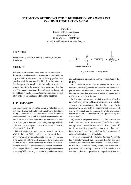
ESTIMATION OF THE CYCLE TIME DISTRIBUTION OF A W AFER FAB BY A SIMPLE SIMULATION MODELOliver RoseInstitute of Computer ScienceUniversity of W¨u rzburg97074W¨u rzburg,GERMANYe-mail:rose@informatik.uni-wuerzburg.deKEYWORDSManufacturing,Factory,Capacity Modeling,Cycle Time, SimulationABSTRACTSemiconductor manufacturing facilities are very complex. To obtain a fundamental understanding of the effects of dispatch and lot release rules on the factory performance based on a full factory model is difﬁcult.In this paper,we therefore present a simple factory model that is intended to show essentially the same behavior as the complete fac-tory.The model consists of the bottleneck workcenter of the full factory model represented in full detail and several delay units for the aggregated remaining machines.1INTRODUCTIONIn a recent paper,we presented a simple wafer fab model that exhibits essential features of a real wafer fab(Rose, 1998).It consists of a detailed model of the bottleneck workcenter and a delay unit that models the remaining ma-chines of the fab.Lots released to the fab model have to cycle through the bottleneck and delay unit repeatedly in order to model the layered nature of semiconductor man-ufacturing(cf.Figure1).This fab model was used to assess the evolution of the Work In Process(WIP)level and cycle time of the fab after recovering from a catastrophic failure,i.e.,a com-plete failure of all bottleneck machines for a long period of ing the proposed model,we were able to repro-duce fab behavior as observed in real semiconductor man-ufacturing facilities.It turned out that the phenomenon of increasing WIP is mainly caused by a combination of thebottleneck workcenterFigure1:Simple factory modeldue-date oriented dispatching and the cyclic nature of the lotﬂow.In the above study,we were not able to obtain real fab measurements to support the parameterization of our sim-ple fab model.In particular,we had to assume that the de-lay time variation lies between the one of a constant and a shifted exponential distribution.In this paper,we present a statistical analysis of the lot intervisit times of the bottleneck workcenter in a realistic semiconductor manufacturing facility.By means of this analysis,we are able toﬁt the parameters of an improved simple fab model,and to compare the cycle time distri-butions of the full fab model with those predicted by the simple model.By means of simple fab models,we intend to foster our basic understanding of the behavior of wafer fabs under the regime of different lot release and dispatch rules.If the simple modeling approaches mimic accurately the full fabs,these models can be applied for the development of new control strategies for wafer fabs.The paper is organized as follows.Section2presents the full factory model,the considered dispatch and load scenarios,and some statistical properties of the full model. In Section3the simple factory model is introduced and parameterized according to the statistical results from Section2.Section4provides a comparison of the cy-cle time distributions of both models for several scenarios and a discussion of the capabilities of the simple factory model.2FULL FACTORY MODELAs test fab for our experiments,we chose the slightly modiﬁed MIMAC fab#6testbed data set that we obtained from Prof.Fowler(MASMLAB,Arizona State Univer-sity,).MIMAC(Mea-surement and Improvement of MAnufacturing Capacity) was a joint project of JESSI/MST and SEMATECH to identify and measure the effects and interactions of ma-jor factors that cause loss in fab efﬁciency(Fowler and Robinson,1995).Fab#6consists of228machines and97operators.It manufactures9types of wafers each of which has more than10layers and requires more than250process steps. The modiﬁed fab produces no scrapped wafers and has only6products because there are3products that do not require the bottleneck workcenter for being processed. With respect to dispatch rules it should be noted that setup avoidance is always used in our experiments.The time be-tween lot starts of each product is constant.We use the Factory Explorer simulation tool to collect the following datasets from the modiﬁed MIMAC#6full fab model(Wright Williams&Kelly,1997).Given a bot-tleneck load and a dispatch rule for all workcenters/tool groups,we record for each product the following delays. We consider the time from lot start until itﬁrst reaches the bottleneck,the start delay,for each cycle separately the time it takes to reenter the bottleneck after leaving it, the cycle delay,and the time from leaving the bottleneck for the last time until having left the fab,theﬁnal delay. For each considered time period several thousand mea-surements are taken.The measured intervals consist of processing times,setup times,and waiting times.Then, for each of the data sets a theoretical distribution is se-lected.The decision is based on Q-Q-plots and sums of squared differences of the measurements’histograms and several distribution candidates.In addition,the autocorre-lation function of each dataset is computed for theﬁrst30 lags.We consider the following four scenarios:FIFO and CR with a bottleneck load of80%and95%,respectively.The dispatch rules are deﬁned as follows.FIFO(First In First Out)The waiting lots are sched-uled in the order of their arrival.This rule does not lead to a reordering of queued lots.CR(Critical Ratio)Each time a lot has to be taken from the queue,the following index is assigned to each of the waiting lots:CRdue date current timeremaining processing time The lot with the smallest index value is chosen for processing.As a consequence,lots that are closer to their due dates are preferred.For a review on dispatch rules see(Wein,1988)or(Ather-ton and Atherton,1995).For each scenario the simulation is run for10years of fab time.Theﬁrst year’s measurements are not consid-ered to avoid initialization bias.We obtain for each time period of interest at least2000measurements.For each scenario more than100distributions have to beﬁtted.To keep the model simple we intend to use only one class of distributions to model all delays.It turns out that the class of shifted Gamma distributions provide the best match among all tested candidates.For each shifted Gamma distribution three parameters have to be estimated:the shape parameter,the scale parame-ter,and the shift parameter.First,we determine the set of parameters that minimizes the squared distance of the empirical density of the measured data and the shifted Gamma density function.Then,while keeping the scale parameter,the two other parameters are recomputed in or-der to obtain the same mean and variance for empirical data and theoretical density function.This method offers the best result with respect to providing a good match in shape of the distributions of the delays while achieving the exact values for mean and variance.As an example, Figure2shows the empirical distribution of theﬁrst cy-cle delay of product1of the CR95%scenario.The other ﬁtted gamma distributions show approximately the same level of accuracy.For the95%scenarios,almost all sequences of mea-surements show considerable correlation.In most cases, the lag-1coefﬁcients of correlation are larger than0.5and the decays of the autocorrelation functions are slower than exponential for at least theﬁrst ten lags.Figure3shows the empirical autocorrelation curve for theﬁrst30lags of the aforementioned sequence of measurements.These correlations originate basically from the fact that subsequent lots of the same product and the same layer,0.010.020.030.040.050.06020406080100120140hoursdata gammaFigure 2:Example distribution of a cycle delay00.10.20.30.40.50.60.7051015202530lagFigure 3:Example correlations of a cycle delay i.e.,the same bottleneck intervisit cycle,see the fab and its machines in roughly the same state.Due to dispatch rules such as FIFO or CR,overtaking of lots is avoided to a large extent.In addition,lots are grouped while waiting for batch completion at batch machines such as oxidation ovens.3SIMPLE FACTORY MODELIn order to predict the cycle time distributions correctly,the model used in (Rose,1998)has to be modiﬁed.The general idea of a detailed model of the bottleneck work-center and delay units representing all other workcenters is kept.The bottleneck model includes the number of ma-chines,the processing times of each product,and the ap-plication of the full fab dispatch rule.There is one delay unit for the time spent by a lot from release to ﬁrst entering the bottleneck work center,one delay unit for the period oftime that it takes from departing the bottleneck machines until reentering the bottleneck queue,and a delay unit for the time from leaving the bottleneck for the last time until ﬁnishing the ﬁnal processing step.The model is depicted in Figure 4.bottleneck workcenterFigure 4:Modiﬁed simple factory modelAll delays are modeled by shifted Gamma distributions that are parameterized as mentioned in Section 2.For each product the delays are determined individually.The same holds for each product’s cycle delays.To model correlated delays,we choose the following approach.If we add two random variables that are Gamma distributed with a common shape parameter the result is Gamma distributed with the same shape parameter and a scale parameter that is the sum of the two single ones (Law and Kelton,1991).Given a sequence of random variables that are distributed for a pos-itive integer .Then,the sumis distributed for .The coefﬁcients ofcorrelation result infor ,and for ,because we keep values and replace just a single value to compute from .This simple approach facilitates a delay model with Gamma distributed delays having a linearly decreasing correlation structure.The modeling of delays with other correlation structures,such as autoregressive processes,while still providing Gamma distributed values is consid-erably more complex than the above method (Cario and Nelson,1996).4RESULTSThe simple factory model is implemented in ARENA 3.01(Kelton et al.,1997).The duration of each run is 10years of simulated time.Measurements taken during the ﬁrst year are cut off.To determine whether both the simple factory model and the full factory model exhibit the same behavior,our primary goal is to match cycle times for each product in mean,variance,and shape of distribution for both models.In the following experiments,lot release and,as a con-sequence,bottleneck loads are exactly the same for both models.We ﬁrst consider FIFO dispatching.In the 80%load scenario the correlations of the delays are low compared to the 95%case.Thus,we used uncorrelated delay units for the simple fab model.Figure 5shows the cycle times of product #1.The histograms of the cycle times for the simple and the full factory models match well.The same holds for all other products.00.0020.0040.0060.0080.010.0120.0140.0160.018550600650700750800hoursfull simpleFigure 5:Product #1cycle times (FIFO 80%)In the FIFO 95%load scenario,the delays are consid-erably correlated with empirical lag-1coefﬁcients of cor-relations ranging from about 0.5up to 0.9.To keep the model simple,we apply two correlation scenarios:mod-erate with a lag-1correlation of 0.66()and strong with a lag-1correlation of 0.9().Without model-ing the correlations the histogram shapes look similar but the mean cycle times are too low.Introducing positive correlation has a clumping effect on the lots because con-secutive lots of the same product have similar delays.It turns out,however,that this lot clumping does not result in higher cycle times as expected.Figure 6depicts the product #1cycle time histograms of the full fab and the simple fab with uncorrelated delays.The histograms for the correlated delays are not shown because they almost match the uncorrelated one.In the following,CR dispatching is considered.The FIFO dispatching at 95%load leads to an average ﬂow factor over all products of about 2.1,where the ﬂow fac-tor is deﬁned as the ratio of average cycle time and raw processing time.The target ﬂow factor for the CR 95%scenario is set to 2.1.This results in shorter cycle times for all but one product and a considerable reduction of00.0020.0040.0060.0080.010.01270075080085090095010001050hoursfull simpleFigure 6:Product #1cycle times (FIFO 95%)variance of cycle times for all products.This is a typi-cal result for switching from FIFO to CR in a wafer fab (Brown et al.,1997).In Figure 7cycle time histograms of product #1under the regime of FIFO and CR are provided.00.0050.010.0150.020.0250.030.03570075080085090095010001050hoursCR FIFOFigure 7:Product #1cycle times (FIFO/CR 95%)Figure 8shows the cycle time histograms of the CR 95%scenario.In contrast to the FIFO scenarios,the shapes of the histogram curves do not match well for ei-ther strength of correlation.This result is caused by a special property of the CR dispatch rule.The application of CR not only completely avoids overtaking of lots of the same product and cycle,such as FIFO does,but also to a large extent overtaking of lots of the same product that are in different cycles,and of lots of different products.Here,lot overtaking is deﬁned as lots being processed earlier at the bottleneck than lots that are closer to their due date.In the full factory model this kind of overtaking only rarely happens because at each machine the lots are processed according to their due dates.In the simple model,however,this reordering0.0050.010.0150.020.0250.030.03565070075080085090095010001050hoursfull simpleFigure 8:Product #1cycle times (CR 95%)0.0050.010.0150.020.0250.030100200300400500600700800900hoursFigure 9:Full factory model histograms of cycle comple-tion timesof lots does only take place at the bottleneck workcenter.Only the effect of overtaking of lots of the same product and cycle is reduced by introducing correlation that leads to lot clumping.The variance reduction effect of CR is visualized in Fig-ure 9and Figure 10.In both cases lots have the same distribution of cycle delays for each cycle,but the shapes of histograms of the periods of time taken from lot start to ﬁnishing a particular cycle are considerably different.In case of full factory with CR,most of the histograms of consecutive cycles are clearly separated (cf.Figure 9)whereas the histograms in the case of simple factory with CR overlap (cf.Figure 10).Due to CR,lots of one product being in the same cycle are grouped together with respect to cycle times in the full factory model.Table 1shows the mean and standard deviation values and of the cycle times of product #1for the consid-ered scenarios.In case of FIFO,the simple factory model values are close to those of the full model.For the CR sce-00.0050.010.0150.020.0250.03100200300400500600700800900hoursFigure 10:Simple factory model histograms of cycle com-pletion timesTable 1:Mean and variance of product #1cycle timesFIFOCRfull simplefull simple95%80%nario,however,the values provided by the simple model are considerably lower than for the full model.5CONCLUSION AND OUTLOOKIn this paper,we presented a simple factory model that is intended to predict the cycle time distributions of the lots in a semiconductor fab and to facilitate the understand-ing of the basic fab behavior under the regime of different dispatching and lot start rules.We considered constant lot release and both FIFO and Critical Ratio (CR)dispatch at different bottleneck loads.The model is well suited to predict the cycle times in the FIFO case.For CR,however,the dispatch rule avoids overtaking of lots with a later due date if other lots with a closer due date are already waiting for a resource to be-come available.This property of CR reduces both mean and variance of the cycle times.The current version of the simple factory model is not capable of avoiding lot overtaking.This results in cycle times that have a higher variance than those of the full factory model.Currently,we consider several correlation scenarioswith respect to their ability to mimic the non-overtaking property of CR dispatch.As a next step it is planned to investigate the appropriateness of the simple model for semiconductor fabs in the presence of complex lot release strategies such as workload regulation(Lawton et al.,1990)or CONWIP(Hopp and Spearman,1991) ACKNOWLEDGEMENTSThe author would like to thank Robert Laufer for his valu-able programming efforts and fruitful discussions. REFERENCESAtherton,L.F.and Atherton,R.W.(1995).Wafer Fab-rication:Factory Performance and Analysis.Kluwer, Boston.Brown,S.,Fowler,J.,Gold,H.,and Sch¨o mig,A.(1997). Measurable improvements in cycle-time-constrained capacity.In Proceedings of the6th International Sym-posium on Semiconductor Manufacturing.Cario,M.C.and Nelson,B.L.(1996).Autoregressive to anything:Time-series input processes for simulation. Operations Research Letters,(19):51–58.Fowler,J.and Robinson,J.(1995).Measurement and im-provement of manufacturing capacities(MIMAC):Fi-nal report.Technical Report95062861A-TR,SEMAT-ECH,Austin,TX.Hopp,W.J.and Spearman,M.L.(1991).Throughput of a constant work in process manufacturing line subject to failures.International Journal of Production Research, 29(3):635–655.Kelton,W.D.,Sadowski,R.P.,and Sadowski,D.A. (1997).Simulation with Arena.McGraw–Hill,New York.Law,A.M.and Kelton,W.D.(1991).Simulation Model-ing&Analysis.McGraw–Hill,New York,2nd edition. Lawton,J.W.,Drake,A.,Henderson,R.,Wein,L.M., Whitney,R.,and Zuanich,D.(1990).Workload regu-lating wafer release in a GaAs fab facility.In Proceed-ings of the International Semiconductor Manufacturing Science Symposium,pages33–38.Rose,O.(1998).WIP evolution of a semiconductor fac-tory after a bottleneck workcenter breakdown.In Pro-ceedings of the Winter Simulation Conference’98. Wein,L.M.(1988).Scheduling semiconductor wafer fab-rication.IEEE Transactions on Semiconductor Manu-facturing,1(3):115–130.Wright Williams&Kelly(1997).Factory Explorer2.3 User Manual.AUTHOR’S BIOGRAPHYOLIVER ROSE is an assistant professor in the Depart-ment of Computer Science at the University of W¨u rzburg, Germany.He received an M.S.degree in applied mathe-matics and a Ph.D.degree in computer science from the same university.He has a strong background in the mod-eling and performance evaluation of high-speed commu-nication networks.Currently,his research focuses on the analysis of semiconductor and car manufacturing facili-ties.He is a member of IEEE,INFORMS,and SCS.。

Reputation and imperfect Information

(page
338)
The intuitive appeal of this line of reasoning has, however, been called the “chain-store paradox” by Selten [24], who demonstrates that it is not supported in a straightforward game-theoretic model. We shall elaborate Selten’s argument later, but the crux is that, in a very simple environment, there is no means by which thoroughly rational strategies in one market could be influenced by behavior in a second, essentially independent market. 253
0022-053
All
l/82/040253-27SO2.00/0
Copyright 0 1982 by Academic Press, Inc. rights of reproduction in any form reserved.
254
KREPS
AND
WILSON
What is lacking, apparently, is a plausible mechanism that connects behavior in otherwise independent markets. We show that imperfect information is one such mechanism. Moreover, the effects of imperfect information can be quite dramatic. If rivals perceive the slightest chance that an incumbent firm might enjoy “rapacious responses,” then the incumbent’s optimal strategy is to employ such behavior against its rivals in all, except possibly the last few, in a long string of encounters. For the incumbent, the immediate cost of predation is a worthwhile investment to sustain or enhance its reputation, thereby deterring subsequent challenges. The two models we present here are variants of the game studied by Selten [24]; several other variations are discussed in Kreps and Wilson 181. The first model can be interpreted in the context envisioned by Scherer: A multimarket monopolist faces a succession of potential entrants (though in our model the analysis is unchanged if there is a single rival with repeated opportunities to enter). We treat this as a finitely repeated game with the added feature that the entrants are unsure about the monopolist’s payoffs, and we show that there is a unique “sensible” equilibrium where, no matter how small the chance that the monopolist actually benefits from predation, the entrants nearly always avoid challenging the monopolist for fear of the predatory response. The second model enriches this formulation by allowing, in the case of a single entrant with multiple entry opportunities, that also the incumbent is uncertain about the entrant’s payoffs. The equilibrium in this model is analogous to a price war: Since the entrant also has a reputation to protect, both firms may engage in battle. Each employs its aggressive tactic in a classic game of “chicken,” persisting in its attempt to force the other to acquiesce before it would itself give up the fight, even if it is virtually certain (at the outset) that each side will thereby incur short-run losses. After reviewing Selten’s model in Section 2, we analyze these two models in Sections 3 and 4, respectively. In Section 5 we discuss our results and relate them to some of the relevant literature. In particular, this issue of the Journal includes a companion article by Milgrom and Roberts ] 131 that explores many of the issues studied here in models that are richer in institutional detail. Their paper is highly recommended to the reader.

mams03

18
System Dynamics and Simulation Basics
System Dynamics
• System
– Collection of Interacting Elements working towards a Goal
• System Elements
– – – – Entities Activities Resources Controls
Simulation Basics
Simulation Basics
• Types of Simulation
– Static/ Dynamic – Stochastic/Deterministic – Discrete Event/Continuous
• Simulating Random Behavior
12
Steps in Simulation -contd.
• Production Runs and Analysis • Documentation/Reporting • Implementation
13
Input Data Representation
• Random Numbers and Random Variates X = (1/) ln( 1- R) • Independent Variables
6
Modeling Structures
• • • • Process-Interaction Method Event-Scheduling Method Activity Scanning Three-Phase Method
7
Advantages of Simulation
• • • • • • • Decision aid. Time stretching/contraction capability. Cause-effect relations Exploration of possibilities. Diagcation of constraints. Visualization of plans.

simulation 形容词

simulation 形容词simulation (形容词) - simulated or imitated closely according to models or patterns1. The flight simulator provided a realistic simulation of flying a fighter jet.飞行模拟器提供了逼真的战斗机飞行模拟体验。

2. The business simulation game allowed participants to experience running a virtual company.这个商业模拟游戏让参与者能够体验经营一个虚拟公司。

3. The virtual reality headset created a simulation of being underwater.这款虚拟现实头盔创造了一种水下的模拟体验。

4. The flight attendant training included a simulation of emergency situations.乘务员培训包括紧急情况的模拟。

5. The simulation exercise helped doctors practice performing surgeries before operating on real patients.模拟训练有助于医生在进行实际手术之前进行实践。

6. The video game provided a simulation of being a professional athlete on the soccer field.这个电子游戏提供了一个模拟身份成为职业足球运动员的体验。

7. The military used a simulation of a battlefield to train soldiers for combat scenarios.军方使用战场模拟训练士兵应对战斗场景。

A survey on modeling and simulation of vehicular networks_ Communications, mobility, and tools

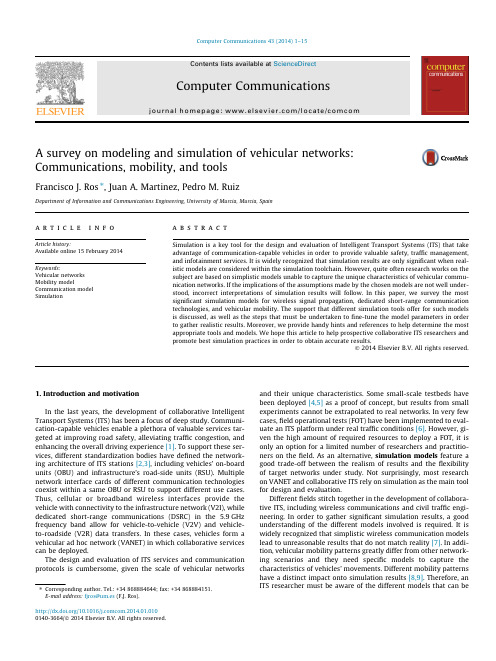
A survey on modeling and simulation of vehicular networks:Communications,mobility,andtoolsFrancisco J.Ros ⇑,Juan A.Martinez,Pedro M.RuizDepartment of Information and Communications Engineering,University of Murcia,Murcia,Spaina r t i c l e i n f o Article history:Available online 15February 2014Keywords:Vehicular networks Mobility modelCommunication model Simulationa b s t r a c tSimulation is a key tool for the design and evaluation of Intelligent Transport Systems (ITS)that take advantage of communication-capable vehicles in order to provide valuable safety,trafﬁc management,and infotainment services.It is widely recognized that simulation results are only signiﬁcant when real-istic models are considered within the simulation toolchain.However,quite often research works on the subject are based on simplistic models unable to capture the unique characteristics of vehicular commu-nication networks.If the implications of the assumptions made by the chosen models are not well under-stood,incorrect interpretations of simulation results will follow.In this paper,we survey the most signiﬁcant simulation models for wireless signal propagation,dedicated short-range communication technologies,and vehicular mobility.The support that different simulation tools offer for such models is discussed,as well as the steps that must be undertaken to ﬁne-tune the model parameters in order to gather realistic results.Moreover,we provide handy hints and references to help determine the most appropriate tools and models.We hope this article to help prospective collaborative ITS researchers and promote best simulation practices in order to obtain accurate results.Ó2014Elsevier B.V.All rights reserved.1.Introduction and motivationIn the last years,the development of collaborative Intelligent Transport Systems (ITS)has been a focus of deep muni-cation-capable vehicles enable a plethora of valuable services tar-geted at improving road safety,alleviating trafﬁc congestion,and enhancing the overall driving experience [1].To support these ser-vices,different standardization bodies have deﬁned the network-ing architecture of ITS stations [2,3],including vehicles’on-board units (OBU)and infrastructure’s road-side units (RSU).Multiple network interface cards of different communication technologies coexist within a same OBU or RSU to support different use cases.Thus,cellular or broadband wireless interfaces provide the vehicle with connectivity to the infrastructure network (V2I),while dedicated short-range communications (DSRC)in the 5.9GHz frequency band allow for vehicle-to-vehicle (V2V)and vehicle-to-roadside (V2R)data transfers.In these cases,vehicles form a vehicular ad hoc network (VANET)in which collaborative services can be deployed.The design and evaluation of ITS services and communication protocols is cumbersome,given the scale of vehicular networks and their unique characteristics.Some small-scale testbeds have been deployed [4,5]as a proof of concept,but results from small experiments cannot be extrapolated to real networks.In very few cases,ﬁeld operational tests (FOT)have been implemented to eval-uate an ITS platform under real trafﬁc conditions [6].However,gi-ven the high amount of required resources to deploy a FOT,it is only an option for a limited number of researchers and practitio-ners on the ﬁeld.As an alternative,simulation models feature a good trade-off between the realism of results and the ﬂexibility of target networks under study.Not surprisingly,most research on VANET and collaborative ITS rely on simulation as the main tool for design and evaluation.Different ﬁelds stitch together in the development of collabora-tive ITS,including wireless communications and civil trafﬁc engi-neering.In order to gather signiﬁcant simulation results,a good understanding of the different models involved is required.It is widely recognized that simplistic wireless communication models lead to unreasonable results that do not match reality [7].In addi-tion,vehicular mobility patterns greatly differ from other network-ing scenarios and they need speciﬁc models to capture the characteristics of vehicles’movements.Different mobility patterns have a distinct impact onto simulation results [8,9].Therefore,an ITS researcher must be aware of the different models that can be/10.1016/com.2014.01.0100140-3664/Ó2014Elsevier B.V.All rights reserved.⇑Corresponding author.Tel.:+34868884644;fax:+34868884151.E-mail address:fjros@um.es (F.J.Ros).employed for each aspect of the simulation environment and how model parameters should be tuned to obtain realistic results.While,traditionally,mobility and network simulators have been developed by different communities for different end users, both tools merge in collaborative ITS.It is of paramount impor-tance that simulations account for realistic vehicles’movements as generated by mobility simulators.Then,network simulators must provide realistic simulation of communication models as the vehicles move according to a given trafﬁc pattern.In some cases,an ITS application inﬂuences the mobility of vehicles.For in-stance,a trafﬁc management service might indicate some vehicles to follow an alternative route to avoid a congested road.To support such scenarios,integrated mobility and network simulations are necessary and can be provided by interfacing existing tools or developing new ones.In this paper,we survey the most signiﬁcant approaches for wireless modeling and mobility modeling in vehicular networks. Speciﬁcally,we describe the models that have been often em-ployed to characterize wireless signal propagation(path loss and fading)in the absence or presence of obstacles,including the sup-port provided in available simulation mon conﬁgura-tions of models parameters for both highway and urban environments are provided when applicable.In addition,we cover the simulation models which are available for the simulation of IEEE802.11p DSRC and related standards.Differences among them are outlined.Regarding vehicular mobility,we brieﬂy review some of the many models that have been proposed for decades and pro-vide references forﬁne-tune calibration of model parameters when high mobility accuracy is required.Furthermore,we summarize the main features of common mobility simulation tools and de-scribe the process to obtain a realistic vehicular scenario.Finally, we discuss the available options for performing integrated mobil-ity and network simulations.We hope this work to help prospec-tive collaborative ITS researchers and promote best simulation practices in order to obtain accurate results.The reminder of this paper is organized as follows.Section2is focused on wireless signals modeling and simulation tools in the context of vehicular networks.Simulation models for DSRC tech-nologies are reviewed in Section3.In Section4,we survey some signiﬁcant vehicular mobility models and different trafﬁc simula-tion packages.The steps to set up a realistic vehicular scenario are also discussed.Section5deals with coupled network and mobility simulations to account for ITS services that inﬂuence the behavior of trafﬁcﬂows.Finally,Section6concludes this article.2.Vehicular wireless communicationUnderstanding the implications of our chosen communication models is key to design appropriate simulation experiments and get insight from their results.In this section we review the most relevant models for vehicular communication systems,as well as the different tools that support them.We highlight the main take-aways that a prospective ITS researcher must keep in mind when conducting a simulation-based study.In addition,valuable information and handy references to help design experiments with different degrees of realism are provided.2.1.Modeling of wireless linksWhen modeling a wireless ad hoc network,one of theﬁrst questions we have to answer is when we can state that a node1u is able to communicate with another node v.In such case,we say that a link exists from u to v.2The simplest approach to model a wireless link is derived from a Uniform Disk Graph(UDG).All nodes are assumed to feature a com-munication range of radius r.In this way,a bidirectional link be-tween u and v exists if and only if j u;v j6r,where jÁj denotes the Euclidean distance.Note that a UDG represents an ideal net-work in the sense that perfect communication occurs up to r dis-tance units from the source.This model does not have into account reception errors which might be provoked by radio inter-ferences.It has been often employed in the literature since it pro-vides a rough estimation of network connectivity in a simple way. However,it is well known that real wireless links do not follow this ideal model at all[11].In order to capture the characteristics of realistic wireless links, signal propagation must be accurately deﬁned(Section2.2).This determines how signal power dissipates as a function of the dis-tance.In the absence of interferences,the receiver will be able to decode the wireless signal,and therefore reconstruct the original message,whenever the signal to noise ratio(SNR)satisﬁes the fol-lowing condition:SNR¼SNP b;where S is the received signal power,N is the noise power,and b is a threshold dependent on the sensitivity of the wireless decoder. Noise represents the undesired random disturbance of a useful information signal.Since wireless medium is shared by the nodes in an ad hoc net-work,transmissions from a node interfere with concurrent com-munications between different nodes.This may cause great disturbance in the resulting signal,so that receivers would not be able to decode the message.In such case,we say that a collision has occurred.Thus,in the most general case,correct reception of a message by a node must satisfy that the signal to interference-noise ratio(SINR)holds the following requirement:SINR¼SIþNP b;where I is the cumulative power of interfering signals.Next we de-scribe some of the commonly employed propagation models for wireless signals,so that the SINR for a given receiver can be computed.2.2.Modeling of wireless signal propagationAs we have seen in the previous subsection,the signal strength at the receiver is lower than when it leaves the transmitter.Several factors contribute to this phenomenon,such as the natural power dissipation as the signal expands,the presence of obstacles which reﬂect,diffract and scatter the original signal,and the existence of multiple paths which may lead to signal cancellation at the recei-ver.The mean signal strength at the receiver as a function of the distance from the transmitter can be estimated by large-scale prop-agation models,while rapidﬂuctuations of the signal at the wave-length scale is better represented by small-scale fading models.The following subsections brieﬂy review the most representative mod-els that are relevant to vehicular wireless communications.They can be classiﬁed according to different criteria[12].In Fig.1,we distinguish among(i)deterministic vs stochastic models,(ii) large-scale path loss vs small-scale fading models,and(iii)whether obstacles(surrounding buildings,the vehicles themselves)are1Throughout this paper,‘node’can be exchanged with‘vehicle’or‘RSU’.2We assume that nodes employ omni-directional antennas.This is the most common scenario,although works on vehicular ad hoc networks with directional antennas have also been undertaken[10].2 F.J.Ros et al./Computer Communications43(2014)1–15explicitly accounted for or not.At the expense of higher computa-tion cost,increased realism is achieved by considering more characteristics of the wireless channel.In order to achieve this, some models build upon simpler ones to provide a more realistic framework for vehicular communications.For a deeper coverage of large-scale and small-scale fading models in general,please refer to[13].rge-scale path lossGiven the transmission power P t,large-scale models predict the received signal power P r as a function of the distance d between transmitter and receiver.The attenuation of the signal strength at the receiver with respect to the transmitter is called the path loss (PL).Regardless the propagation model we employ to obtain P r,the path loss can be computed(in dB)as in the following expression:PLðdÞ¼10log10P t P rThe Friis’free space propagation model[14]assumes the ideal condition that there is just one clear line-of-sight(LOS)path be-tween sender and receiver.If we consider isotropic antennas and nodes located in a plane,this model represents the communication range as a circle around the transmitter.Friis proposed the follow-ing expression to compute P r:P rðdÞ¼P t G t G r k2ð4pÞ2d2L;ð1Þwhere G t and G r are the antenna gains of the transmitter and recei-ver respectively,L P1is the system loss(because of electronic cir-cuitry),k is the signal wavelength,and P r is measured in the same units as P t(usually W or mW).As you can see,signal strength de-cays as a quadratic power law of the distance.In typical communications within a vehicular network,ideal conditions to apply the Friis model are rarely achieved.For in-stance,signal reﬂection is not being considered.The two-ray ground reﬂection model[13]provides more accurate predictions by explicitly accounting for both the direct path between sender and receiver and the ground-reﬂected path.For large distances, the following expression estimates the received signal strength: P rðdÞ¼P t G t G r h2th2rd4L;ð2Þwhere h t and h r are the heights of the transmit and receive anten-nas,respectively,and P r is measured in the same units as P t(usually W or mW).Note that according to Eq.(2),when transmitter and receiver are far away(d)ﬃﬃﬃﬃﬃﬃﬃﬃﬃh t h rp)the power decays with the distance raised to the fourth power(much faster fall than in free space). In addition,the path loss becomes independent of the signal fre-quency.The former conclusions do not hold for a short distance d,in which case a different expression must be used to compute P r.A common model employed in such cases is the Friis’free space propagation.For instance,such approach can be found in both the ns-2and ns-3network simulators.Thus,a cross-over distance d c is calculated:when d<d c,Eq.(1)is employed;when d>d c,Eq.(2)is used;at the cross-over distance d c,Friis and two-ray ground mod-els provide the same result.Therefore,d c can be computed as follows:d c¼4p h t h rkNote that for the5.9GHz DSRC band for vehicular communica-tions,and assuming that antennas are mounted on cars’roofs at1.5 meters high,d c%556m.This means that if you are employing the two-ray ground model in an ns-2or ns-3simulation of a IEEE WAVE/802.11p vehicular ad hoc network,communications be-tween vehicles far away less than556m will experience a qua-dratic power decay typical of free space communications.This could lead to non-accurate simulationresults. Fig.1.Taxonomy of wireless signal propagation models for V2V/V2R communications.In any case,the former models are not able to capture the dif-ferent subtleties of wireless communications in general,and vehic-ular environments in particular.Therefore,most models employed in practice follow an empirical approach in which analytical expressions for the path loss areﬁtted according to a set of mea-surements performed in the target scenario.Such expressions approximate the signal strength at an arbitrary distance d by tak-ing as input the signal strength at a reference close distance d0. P rðd0Þcan be either empirically determined or computed according to the free space model(Eq.(1)).For DSRC vehicular communica-tions,commonly employed values for d0are10m[15]and1m [16].The log-distance path loss model[13]includes a path loss expo-nent c that indicates the rate at which the path loss increases with the distance:P rðdÞ¼P rðd0ÞÀ10c log10dd0;ð3Þwhere P r is measured in dB.Given a set of measurements,the path loss exponent c can beﬁtted to let Eq.(3)approximate the real data set.In practice,dual-slope piecewise-linear models like the one in Eq.(4)provide a betterﬁt.Such model has been employed to rep-resent large-scale path loss in highways[15]by adjusting its parameters according to a set of experiments carried out at highway 101in the Bay Area[17].Afterwards,this dual-slope log-distance model was implemented within ns-2[16]and later on integrated within the ofﬁcial simulator codebase(starting from ns-2.34).P rðdÞ¼P rðd0ÞÀ10c1log10d dd06d6d cP rðd0ÞÀ10c1log10d cÀ10c2log10dcd>d c8><>:ð4ÞSo far,all reviewed models ignore the fact that two receivers at the same distance d from the transmitter could sense very different signal strengths depending on the environment the signal encoun-ters on its path.Different measurements have shown that the sig-nal strength(in dB)is random and log-normally distributed about the mean distance-dependent value.Therefore,log-normal shad-owing models better capture this fact:P rðdÞ¼P rðd0ÞÀ10c log10dd0þX r;ð5Þwhere X r is a zero-mean normally distributed random variable with standard deviation r.By means of sets of experiments,parameters c and r can be obtained via linear regression,adjusting the model to produce realistic random values for a given scenario.Also in this case,more accurate results have been found by using dual-slope piecewise-linear models such as the one in Eq.(6).This model has been employed for urban scenarios[18],where the authors con-ducted two sets of experiments in Pittsburgh.The obtained conﬁg-uration has been employed afterwards[19]to perform vehicular simulations in ns-2.3P rðdÞ¼P rðd0ÞÀ10c1log10dþX r1d06d6d cP rðd0ÞÀ10c1log10d c dÀd>d c10c2log10dcþX r28>>>><>>>>:ð6ÞIn order to provide the reader with a handy reference,Table1 summarizes the conﬁguration of the main path loss models that have been employed for characterizing vehicular networks,both in highway and urban scenarios.Fig.2shows the impact of free space,two-ray ground and single-slope log-normal shadowing(ur-ban environment,third row of Table1)on vehicular communica-tions at the5.9GHz DSRC band.The results have been obtained in an interference-free unobstructed scenario with IEEE802.11p communications at3Mbps.The transmission power is set to 20dB,and antennas are mounted at 1.5m height.Destination vehicles are from10m to2000m away from the source,which is-sues500broadcast frames.For each one,we record the power level each receiver senses the frame,including whether it can be suc-cessfully decoded.Note that free space and two-ray ground models provide the same power loss up to the cross-over distance d c(Fig.2(a))in com-mon implementations of these simulation models.In addition, both approaches feature a non-realistic deterministic radio range, Table1Conﬁguration of path loss models for vehicular networks.Legend:P reference to model proposal.S reference to model usage in simulation.Scenario Model Parameters P SHighway dual-slope c1¼1:9c2¼3:8[17]log-distance d c¼200m[16]d c¼80m[15]Urban log-normal c¼2:75r¼5:5[18]Urban log-normal c¼2:32r¼7:1[18]Urban dual-slope c1¼2:1c2¼3:8[18]log-normal r1¼2:6r2¼4:4d c¼100mUrban dual-slope c1¼2c2¼4[18][19]log-normal r1¼5:6r2¼8:4d c¼100m(a)Power loss4006008001000120014001600Distance (m)Free spaceTwo−ray groundLog−normal(b)Reception PDFFig.2.Path loss models for vehicular DSRC.3Code available a t ht tp://masimum.in f.um.es/fjrm/develo pm en t/lognormalnakagami6.4 F.J.Ros et al./Computer Communications43(2014)1–15while the log-normal model provides a non-deterministic radio range.This leads to very distinct frame reception probabilities,as can be observed in Fig.2(b).Suchﬁgure shows the probability density function(PDF)of successfully decoding a frame with respect to the distance between sender and receiver.In other words,this‘‘Reception PDF’’characterizes the likelihood that the resulting SINR at the receiver is enough to recover the original frame given the sensitivity of the decoder.While deterministic models offer a binary probability distribution in the absence of interference(frames are always decoded if the distance is below the effective communication range,and not decoded otherwise), stochastic approaches introduce randomness typical of wireless communications.The main take-aways from this subsection can be summarized as:Conditions to convey signiﬁcant simulation results from free space and two-ray ground simulation models are rarely(if ever) achieved in practice for vehicular networks.Log-normal path loss models capture the randomness that log-distance models lack.Usually,multi-slope models provide a betterﬁt than single-slope ones.Whatever the path loss model employed,it must beﬁne-tuned to the particular vehicular scenario(highway,urban)under evaluation.2.2.2.Small-scale fadingPath loss models discussed so far do not capture the effect of the multiple waves of a signal that arrive at the receiver through differ-ent paths.Since the traveled distance is different for each wave,as well as the environment it traverses,each version of the original signal reaches the receiver with different amplitude at a different time instant.In addition,if the transmitter/receiver is in motion as it is the case in vehicular networks,the Doppler effect also causes frequency dispersion with respect to the original signal.These aspects make the receiver face a heavily distorted version of the original signal.There are abrupt changes in amplitude and phase that can be modeled by means of small-scale fading models. Such kind of fading occurs at the scale of a wavelength,and it might be the dominant component in a severe multi-path environ-ment like the one encountered in vehicular networks.In order to account for small-scale fading,we usually rely on statistical distributions that model the envelope of the signal over time[13].The Ricean distribution models the amplitude of a mul-ti-path envelope when there exists a stronger wave with LOS be-tween transmitter and receiver.As the distance between sender and destination increases in the 5.9GHz band,the probability density function of the signal amplitude is better captured by the Rayleigh distribution.In case there is no line-of-sight(NLOS), higher-than-Rayleigh fading is observed(the Weibull distribution can be a goodﬁt in such case[20]).In general,the Nakagami distribution[21]is able to capture different severities of fading depending on the chosen parameters. In fact,Ricean fading can be approximated by Nakagami,Rayleigh fading can be seen as a special case of the Nakagami model,and higher-than-Rayleigh fading can be modeled with Nakagami.This distribution approximates the amplitude of the wireless signal according to the following probability density function fðx;l;xÞ.fðx;l;xÞ¼2l l x2lÀ1x l CðlÞeÀl x2x;ð7Þwhere l is a shape parameter,x¼E½x2 is an estimate of the aver-age power in the fading envelope,and C is the Gamma function. Therefore,x can be computed by employing any of the path loss models that we discussed above.If l¼1,Rayleigh fading is obtained(higher-than-Rayleigh fading for l<1,and less severe fading for l>1).Given that signal amplitude is Nakagami-distributed with parameters l;xðÞ,signal power obeys a Gamma distribution with parametersðl;x lÞ.A set of experiments conducted at highway101in the Bay Area[17]were employed toﬁt this model.Estimate x is computed by means of the dual-slope log-distance model discussed in the previ-ous subsection.For a betterﬁt of the data,distances between sen-der and receiver are grouped in a set of bins and differentﬁts for parameter l are estimated on a per-bin basis.Table2shows the parameters employed in two different highway setups.The Nakagami fading model has also been used for urban sce-narios.In the Pittsburgh experiments[18],x is calculated by means of log-normal path loss models(both single-slope and dual-slope).The value of parameters l on a per-bin basis on two different data sets are provided in Table2.This model is available for simulation as a separate patch for the ns-2network simulator.3 Fig.3compares the power loss and reception probability of high-way(ﬁrst row of Table2)and urban(fourth row of Table2)models in DSRC(same setup as in the otherﬁgures of this section).Note the higher dispersion that fading models provoke with respect to large-scale path loss(Fig.3(a)and(c)),as well as the higher chal-lenge that urban environments impose on vehicular communica-tions(Fig.3(b)and(d)).Fig.4shows the cumulative density function(CDF)of the reception probability in IEEE802.11p when different path loss and fading models are employed in simulation. Suchﬁgure summarizes the results we have seen so far.Speciﬁ-cally,deterministic path loss models are shown to give aﬁxed communication range,which is lower for two-ray ground than free space given that the former models a higher power decay beyond the cross-over distance.On its hand,the log-normal path loss mod-el provides a probabilistic communication range with higher reception likelihood at short distances than at long distances. When small-scale fading is also taken into account,the effective communication range decreases(the reduction is higher in urban scenarios than in highways).The main take-aways from this subsection are:Small-scale fading is the dominant component in dynamic multi-path scenarios like those comprised of communicating vehicles.Therefore,it must be taken into account to convey realistic simulation results.The Nakagami model is general enough to capture different lev-els of fading.Table2Conﬁguration of the Nakagami fading model for vehicular networks.Legend:P reference to model proposal.S reference to model usage in simulation.Scenario x l P SHighway Dual-slope l1¼1:5forð0;80 m[17][19] Log-distance l2¼0:75otherwiseHighway Dual-slope l1¼3forð0;50 m[15][15] Log-distance l2¼1:5forð50;150 ml3¼1otherwiseUrban Log-normal l1¼4:07forð0;5:5 m[18]l2¼2:44forð5:5;13:9 ml3¼3:08forð13:9;35:5 ml4¼1:52forð33:5;90:5 ml5¼0:74forð90:5;230:7 ml6¼0:84forð230:7;588 mUrban Log-normal l1¼3:01forð0;4:7 m[18][19]l2¼1:18forð4:7;11:7 ml3¼1:94forð11:7;28:9 ml4¼1:86forð28:9;71:6 ml5¼0:44forð71:6;177:3 ml6¼0:32forð177:3;439 mF.J.Ros et al./Computer Communications43(2014)1–155A better ﬁt is obtained if different distance bins between sender and receiver are considered.Whatever the fading model employed,it must be ﬁne-tuned to the particular vehicular scenario (highway,urban)under evaluation.2.2.3.Propagation through obstaclesThe former models do not consider obstacles in an explicit way.Given that many of them consist of stochastic processes ﬁne-tuned according to real experiments,the effect of obstacles that reﬂect,diffract and scatter the original signal is incorporated in an indirect way.However,they do not accurately cover the shadowing of the signal by a given obstacle between two vehicles,since the environ-ment map is not incorporated into the model.Therefore,different works have focused on explicitly account-ing for the impact of obstacles into vehicular communications.Obstacles reduce channel congestion at the cost of a greater (more realistic)number of NLOS situations.This also fosters the appear-ance of hidden terminals,challenging the performance of medium access control schemes.Given the existence of numerous obstacles in real vehicular communication scenarios,they should be consid-ered in simulations since they have a great impact onto the accu-racy of simulation results.Ray tracing techniques have been employed to accurately ac-count for the effect of obstacles in wireless communications [22].However,traditional ray tracing is not appropriate for the simula-tion of vehicular networks due to the high processing requirements it imposes.The approach is not able to scale to large networks.Hence,different works have proposed simpliﬁed ray tracing tech-niques that employ pre-processing steps to reduce the simulation time without heavily impacting the accuracy of the results.Along these lines,a general methodology for generating urban channel models for a given 3D map was proposed recently [23].Nevertheless,simpler solutions are often employed in practice.For instance,the ns-2simulator incorporates a so-called shadow-ing visibility model which actually consists of two log-normal models that can be independently conﬁgured.One of them is used when there is LOS between the communicating entities,and the other is employed for NLOS cases.In order to determine what mod-el shall be used for a given transmission,the user must provide a bitmap ﬁle that represents the obstacles in the simulation scenario.The former approach is hard to generalize because it does not account for the number of traversed obstacles,their size,and their shape.In general,it is better to rely on a path loss model and com-pute the extra attenuation which is due to the obstacles which are in the path of the signal.Such scheme is adopted by the inexpen-sive empirical model [24]for urban simulation,in which the extra loss L o is related to the number of times n the border of a obstacle is(a)Power loss -Urban(b)Power loss -Highway vs Urban05001000150020000.511.522.533.5Distance (m)Urban path loss Urban path loss + fading(c)Reception PDF -Urban 020040060080010001200140000.511.522.533.5Distance (m)Highway Urban(d)Reception PDF -Highway vs UrbanFig.3.Fading models for vehicular DSRC.6 F.J.Ros et al./Computer Communications 43(2014)1–15。

预测和控制森林火灾模型

5
5 5 6 7 7 9 9 13 16 18 18 19 20 20 21
6
Model to Reduce Loss of Forest Fire .................................. 16
6.1 Merchant Model ............................................................... 6.1.1 Construction of Merchant Model . . . . . . . . . . . . . . . 6.1.2 Result of Merchant Model . . . . . . . . . . . . . . . . . . . 6.2 Ecology model.................................................................. 6.2.1 Construction of Ecological Model . . . . . . . . . . . . . . 6.2.2 Result of Ecological Model . . . . . . . . . . . . . . . . . .
8 9
Strengths and Weaknesses ................................................. 24 References .......................................................................... 24
1.1 Background ..................................................................... 1.2 Problem Description .......................................................... 3 3

有限元仿真的英语

有限元仿真的英语Finite Element SimulationThe field of engineering has seen a remarkable evolution in recent decades, with the advent of advanced computational tools and techniques that have revolutionized the way we approach design, analysis, and problem-solving. One such powerful tool is the finite element method (FEM), a numerical technique that has become an indispensable part of the modern engineer's toolkit.The finite element method is a powerful computational tool that allows for the simulation and analysis of complex physical systems, ranging from structural mechanics and fluid dynamics to heat transfer and electromagnetic phenomena. At its core, the finite element method involves discretizing a continuous domain into a finite number of smaller, interconnected elements, each with its own set of properties and governing equations. By solving these equations numerically, the finite element method can provide detailed insights into the behavior of the system, enabling engineers to make informed decisions and optimize their designs.One of the key advantages of the finite element method is its abilityto handle complex geometries and boundary conditions. Traditional analytical methods often struggle with intricate shapes and boundary conditions, but the finite element method can easily accommodate these complexities by breaking down the domain into smaller, manageable elements. This flexibility allows engineers to model real-world systems with a high degree of accuracy, leading to more reliable and efficient designs.Another important aspect of the finite element method is its versatility. The technique can be applied to a wide range of engineering disciplines, from structural analysis and fluid dynamics to heat transfer and electromagnetic field simulations. This versatility has made the finite element method an indispensable tool in the arsenal of modern engineers, allowing them to tackle a diverse array of problems with a single computational framework.The power of the finite element method lies in its ability to provide detailed, quantitative insights into the behavior of complex systems. By discretizing the domain and solving the governing equations numerically, the finite element method can generate comprehensive data on stresses, strains, temperatures, fluid flow patterns, and other critical parameters. This information is invaluable for engineers, as it allows them to identify potential failure points, optimize designs, and make informed decisions that lead to more reliable and efficient products.The implementation of the finite element method, however, is not without its challenges. The process of discretizing the domain, selecting appropriate element types, and defining boundary conditions can be complex and time-consuming. Additionally, the accuracy of the finite element analysis is heavily dependent on the quality of the input data, the selection of appropriate material models, and the proper interpretation of the results.To address these challenges, researchers and software developers have invested significant effort in improving the finite element method and developing user-friendly software tools. Modern finite element analysis (FEA) software packages, such as ANSYS, ABAQUS, and COMSOL, provide intuitive graphical user interfaces, advanced meshing algorithms, and powerful post-processing capabilities, making the finite element method more accessible to engineers of all levels of expertise.Furthermore, the ongoing advancements in computational power and parallel processing have enabled the finite element method to tackle increasingly complex problems, pushing the boundaries of what was previously possible. High-performance computing (HPC) clusters and cloud-based computing resources have made it possible to perform large-scale, multi-physics simulations, allowing engineers to gain deeper insights into the behavior of their designs.As the engineering field continues to evolve, the finite element method is poised to play an even more pivotal role in the design, analysis, and optimization of complex systems. With its ability to handle a wide range of physical phenomena, the finite element method has become an indispensable tool in the modern engineer's toolkit, enabling them to push the boundaries of innovation and create products that are more reliable, efficient, and sustainable.In conclusion, the finite element method is a powerful computational tool that has transformed the field of engineering. By discretizing complex domains and solving the governing equations numerically, the finite element method provides engineers with detailed insights into the behavior of their designs, allowing them to make informed decisions and optimize their products. As the field of engineering continues to evolve, the finite element method will undoubtedly remain a crucial component of the modern engineer's arsenal, driving innovation and shaping the future of technological advancement.。

Simulation_of

Simulation of drape behaviour of fabrics 201Simulation of drape behaviour of fabricsHartmut Rödel, Volker Ulbricht, Sybille Krzywinski,Andrea Schenk and Petra FischerDresden University of Technology, Dresden, Germany IntroductionIn the textile and clothing industries, because of the increasingly individual and customer-oriented production, the sample collections of the firms extend more and more, whereas the quantities for the production decrease. At present, the stage of product development and product preparation of clothes requires approximately three times the stage of consumption. In order to compensate the resulting greater efforts in the product preparation and to react more quickly and flexibly to latest fashion, the use of complex CAD-CAM solutions is a must.Today there exist a lot of design programs with various software tools, a wide choice of designing functions are at the disposal of the designer. Connected with sketching-systems, so called two-and-a-half dimensional presentation programs can give an optical impression of how the colours, motifs and materials look on a scanned model. Steps of production preparation such as pattern construction, grading system, pattern planning and pattern optimization and the automated cutting are realized by computer assistance[1].However, of the CAD-systems available on the market (with two exceptions) the systems work only two-dimensionally and the material behaviour and the material parameters are not taken into account.Both these aspects are required for the three-dimensional display of a model with regard to the draping in order to give the designer and model maker a real impression of the model. The three-dimensional display of a two-dimensional pattern construction on a dummy or vice-versa, a development of a three-dimensionally constructed model into the two-dimensional level, would be the optimal possibilities to examine the correct fitting and the form of a model,when the specific material parameters are taken into account.Consequently, the main focus in international research is to investigate the fundamentals of three-dimensional handling of fabrics. For that, a prerequisite is the implementation of algorithms for the simulation of draping of ready-made clothes. The specific material parameters such as the significant material parameters must be taken into consideration. Therefore, more detailed treatment of physical and mechanical properties and their correct mathematical and physical formulation is of interest.This paper is the result of an interdisciplinary research project of the Institute for Mechanics of Solids and the Institute for Textile and Ready-Made Clothing Technique at Dresden University of Technology. It is the aim of this International Journal of Clothing Science and Technology,Vol. 10 No. 3/4, 1998, pp. 201-208,MCB University Press, 0955-6222IJCST 10,3/4 202project to describe and simulate the deformation behaviour of flexural fabrics (especially of woven fabrics). The deformation theory developed in the Institute for Mechanics of Solids and its application for fabrics is utilized as a practicable approach for the simulation of the drape behaviour. Investigations on the description of the material behaviour and of its properties are a further necessary focal point.Drape behaviourIn the mechanical consideration of deformability of fabrics, on principle, two directions are distinguished. The first one deals with the deformational behaviour of fabrics when covering defined surfaces. This application requires a nearly wrinkle free draping of the fabric, as for example when upholstering. Here, the extensibility, i.e. the force-extension relation in case of tensional strain with the corresponding modulus, are significant material parameters. There is a large number of research works in this field.The second one is the drape behaviour of the fabric. The behaviour of non-resistance of fabrics to bending without external force only under the influence of the true specific weight results in a three-dimensional deformation. A possibility to determine objectively the drape behaviour is the draping experiment (Figure 1) carried out using the drape meter developed by Cusick[2] and the calculation of the resulting drape coefficient D in percent.The drape image is characterized by the area, the form and amplitude of the folding, the number of foldings and their position with regard to warp and weft direction. Figure 2 shows two drape images of different woven fabrics.According to Cusick, the drape coefficient is defined by the surface relations of the drape image, the supporting disk and the surface of the cut. So far, many planimetering activities were required. The other characteristic features are not taken into account. For the more efficient evaluation of the tests, the drapemeter measuring device was coupled with a video camera and image processing systems. This measuring method was developed by the Department of TextilesFigure 1.Drape experimentSimulation of drape behaviourof fabrics203of the University of Gent, as reported in [3]. Hence, the previous subjective errors made when measuring were minimized and the drape coefficient was determined within considerably less time. By image processing, new possibilities of evaluation of the drape image were created.Fabrics are classified on the basis of the drape coefficient. A high drape coefficient indicates a small deformation whereas a small drape coefficient marks great deformations and more waves. For these deformations, the specific material properties of the fabric are decisive.To simulate the drape behaviour, so far, mainly fabrics were investigated, because they can be simulated most simply, they are predominant in outer garments and the total testing technique described at present is mainly oriented to fabrics. Therefore, our investigations only refer to fabrics. The fabrics geometry is defined by the fabrics parameters such as weave structure, the number of warp/weft nodes, the fineness of threads, the density of threads in warp and weft. The often viscoelastic behaviour of the material is determined by the material (the fibrous material used), the properties of the individual fibre and by the fabrics geometry. In the three-dimensional deformation investigated in greater detail by Amirbayat and Hearle[4] as double or complex curvature, for the deformation bending and shear properties are decisive. Bending stiffness of fabrics is mainly based on the stability of fibres in the thread. Shear stiffness is a unit of measurement of the ease with which threads are gliding across each other at deformation. For both properties, the thread spacing and crimp in the structure of the fabric is decisive.Besides the bending stiffness and shear stiffness, the drape behaviour of a fabric is determined by the weight/unit area, whereas properties of compression of the surface (friction and roughness) and extension properties have no considerable influence.At present, a system of devices developed according to Kawabata[5] is used internationally for the investigation of mechanical characteristics of fabrics. This system includes measuring devices which are mainly suitable for Figure 2.Drape image D = 60.0% D = 37.9%IJCST 10,3/4 204measuring insignificant quantities of compression, friction and roughness, of bending stiffness and extension.Geometric fundamentalsThe basis for the determination of the drape behaviour is a geometric model adapted to the drape test and shown in Figure 3.Two configurations are related – the non-deformed configuration and the deformed configuration – where the independent values of the model are purely geometric values.Kinematic assumption of the illustration without strains is taken into consideration in the formula for the geometric description of the deformed configuration[6].To describe the geometric model, independent boundary curves are introduced with the local vectors and →r0(– v) and→r1(v);(1)(2) Both local vectors are in one plane z= constant each, in a distance of h to each other. The ruled surface;(3) is formed with the standardized local vector;(4) and the coordinate u∈[0,h]. Functional dependence of the parameters –v=–v(v)of the boundary curves should be determined in such a way that the ruledSimulation of drape behaviourof fabrics 205surface becomes a torse. When the Gauss curvature is zero, the special condition of torse which is adapted to the problem is:(5)with(5a)Analysing equation (5), two surfaces exist of which the deformed geometry is composed – a tangent surface and a conical surface (Figure 3).According to (1) for the vectors →r 0and →r 1various equations can be set up.One possibility is the description of the boundary curves by the following functions (Figure 4):(6)(7)withAs a result, the description of the surface is ensured as required to simulate the drape behaviour. By the function f n (v), a waviness is defined which is superimposed to the lower boundary curve.Calculation of the isometric mapping with constant lengths of the three-dimensional geometry results from the condition that the quadratic lineIJCST 10,3/4 206elements of the three-dimensional and the two-dimensional geometry are identical[7].To simulate the real experiment two constraints prove to be nessesary. Material equation and potentialFor the description of the material properties isotropic, linear-elastic material behaviour is taken as a basis. In the description of surfaces without strains, deformation takes place exclusively by change of curvature of the surface. Only bending moments occur which are linked with the change of curvature κby bending stiffness B. For the solution, the principle of the minimum of the elastic total potential is taken as a basis. It is assumed that the fabric specimen comes down from the planar starting position into that state, where there is a minimum elastic total potential. The task to determine the extreme value for the elastic total potential together with strain energy Wfand external energy Wa can be set up as follows[8]:(8) As the model chosen was introduced as a simply curved one and without strains for strain energy follows:(9) withAnalogously to the assumptions, the integral includes only bending parts. Surfaces without strains are neglected deliberately in order to exclude that when calculating energy, these parts will be predominant caused by numeric inaccuracies with regard to strain energy and the results are distorted.During the drape test, no external forces or momentums occur. Consequently,external energy Wais determined only from the own weight of the material. It is introduced with:(10) with(10a) where by z the difference of the vertical distance of both configurations is designated. The variable F ga is the force of weight per unit area determinedexperimentally. The elastic total potential:Simulation ofdrape behaviourof fabrics207(11)with the parameters to be varied of the radius of the lower boundary curve r 1,amplitude of wave a , number of waves, and overhanging h for the description of the deformed geometry. The minimum is determined by computer assistance and by means of a searching strategy according to Gauss-Seidel.SummaryIn Figure 5, the three-dimensional description of the drape is shown which is generated by means of the simulation model presented. It is in good coincidence with the experiment concerned (Figure 1).In the future the research work has the aim to improve the description of the material behaviour. Therefore it is necessary to consider in the model the shear stiffness too.Summarizing it can be stated that when compared with FEM, a minimum of independent values is sufficient to reach an efficient basic approach of the problem[9]. In addition, very much calculation time can be saved with this method.References1.Kirchdörfer, E. and Mecheels, J., “Wohin steuert CAD in der Bekleidungsindustrie?”,Bekleidung und Wäsche, Vol. 14, 1987, pp. 8-15.2.Cusick, G.E., “The measurement of fabric drape”, Journal of the Textile Institute, Vol. 59No. 6, 1968, pp. 253-60.3Vangheluwe, L. and Kiekens, P. “Time dependence of the drape coefficient of fabrics”,International Journal of Clothing Science and Technology, Vol. 5 No. 5, 1993, pp. 5-8.4.Amirbayat, J. and Hearle, J. “The anatomy of buckling of textile fabrics, drape and conformability”, Journal of the Textile Institute,Vol. 82 No. 1, 1989, pp. 51-70.5.Kawabata, S. and Niwa, C. “Fabric performance in clothing and clothing manufacture”,Journal of the Textile Institute,Vol. 80 No. 1, 1989, pp. 19-50.behaviourIJCST 10,3/4 ndgraf, G., Modler, K.-H., Ulbricht, V. and Ziegenhorn, M., “DifferentialgeometrischeBeschreibung abwickelbarer Flächen”, Informationstechnik it, Vol. 33 No. 2, 1991, pp. 77-82.7.Kreyszig, E., Differentialgeometrie,Akademische Verlagsgesellschaft Geest & Portig K.-G.,Leipzig, 1957.ndgraf, G., Ulbricht, V., Nestler, R. and Krzywinski, S., “Möglichkeiten derÜbertragbarkeit der Methode der doppelt gekrümmten Flächen und der im Maschinenbau gewonnenen Ergebnisse auf die Konfektionsindustrie”, Wissenschaftl. Zeitschrift der TU Dresden, Vol. 44 No. 6, 1992, pp. 79-85.9.Schenk, A., “Berechnung des Faltenwurfs textiler Flächengebilde”, TU Dresden,Dissertation, 1996.。

团购方面外文翻译

Segmenting uncertain demand in group-buying auctions 原文：Demand uncertainty is a key factor in a seller’s decision-making process for products sold through online auctions. We explore demand uncertainty in group-buying auctions in terms of the extent of low-valuation demand and high-valuation demand. We focus on the analysis of a monopolistic group-buying retailer that sells products to consumers who express different product valuations. We also examine the performance of a group-buying seller who faces competitive posted-price sellers in a market for the sale of the same products, under similar assumptions about uncertain demand. Based on a Nash equilibrium analysis of bidder strategies for both of these seller-side competition structures, we are able to characterize the group-buying auction bidders’ dominant strategies. We obtained a number of interesting findings. Group-buying is likely to be more effective in settings where there is larger low-valuation demand than high-valuation demand.Keywords: Consumer behavior, bidding strategy, demand uncertainty, economic analysis, electronic markets, group-buying auctions, market mechanism, posted-price mechanism, simulation, uncertainty risk.The development of advanced IT makes it possible to use novel business models to handle business problems in new and innovative ways. With the growth of the Internet, a number of new electronic auction mechanisms have emerged, and auctions are generally known to create higher expected seller revenue than posted-prices whenthe cost of running an auction is minimal or costless (Wang 1993). Some of the new mechanisms we have seen include the online Yankee and Dutch auctions, and the “name-yourown-price” and “buy-it-now” mechanisms. An example is eBay’s Dutch auction for the sale of multiple items of the same description. Another of these new electronic market mechanisms that we have observed is the group-buying auction, a homogeneous multi-unit auction (Mitchell 2002, Li et al. 2004).Internet-based sellers and digital intermediaries have adopted this market mechanism on sites such as () and (). These sites offer transaction-making mechanisms that are different from traditional auctions. In traditional auctions, bidders compete against one another to be the winner. In group-buying auctions, however, bidders have an incentive to aggregate their bids so that the seller or digital intermediary offers a lower price at which they all can buy the desired goods (Horn et al. 2000). McCabe et al. (1991) have explored multi-unit Vickrey auctions in experimental research, however, they did not consider the possibility of stochastic bidder arrival or demand uncertainty.Based on a Nash equilibrium analysis of bidder strategies for a monopolist seller and a competitive seller, we are able to characterize the group-buying auction bidders’ symmetric and dominant strategies. We find that group-buying is likely to be more effective in settings where there is larger low-valuation demand than high-valuation demand. Thus, the structure of demand at different level of willingness-to-pay by consumers matters. This has relevance to the marketplace for new cameras, next-generation microprocessors and computers, and other high-valuation goods. We obtained additional results for the case of continuous demand valuations, and found that there is a basis for the seller to improve revenues based on the effective design of the group-buying auction price curve design.THEORYThe model for the group-buying auction mechanism with uncertain bidder arrival that we will develop spans three streams of literature: demand uncertainty, consumer behavior and related mechanism design issues; auction economics and mechanism design theory; and current theoretical knowledge about the operation of group-buying auctions from the IS and electronic commerce literature.Demand Uncertainty, Consumer Behavior and Mechanism DesignDemand uncertainties typically are composed of consumer demand environment uncertainty (or uncertainty about the aggregate level of consumer demand) and randomness of demand in the marketplace (reflected in brief temporal changes and demand shocks that are not expected to persist). Consumer uncertainty about demand in the marketplace can occur based on the valuation of products, and whether consumers are willing to pay higher or lower prices. It may also occur on the basis of demand levels, especially the number of the consumers in the market. Finally, there are temporal considerations, which involve whether a consumer wishes to buy now, or whether they may be sampling quality and pricing with the intention of buying later. We distinguish between different demand level environments. In addition, it is possible that these consumer demand environments may co-exist, as is often the case when firms make strategies for price discrimination. This prompts a seller to consider setting more than one price level, as we often see in real-world retailing, as well as group-buying auctions.Dana (2001) pointed out that when a monopoly seller faces uncertainty about the consumer demand environment, it usually will not be in his best interest to set uniform prices for all consumers. The author studied a scenario in which there were more buyers associated with high demand and f ewer buyers associated with low demand. In the author’s proposed price mechanism, the seller sets a price curve instead of a single price, so as to be able to offer different prices depending on the different demand conditions that appear to obtain in the marketplace. It may be useful in such settings to employ an automated price-searching mechanism, which is demonstrated to be more robust to the uncertain demand than a uniform price mechanism will, relative to expected profits. Unlike Dana’s (2001) work th ough, we will study settings in which there are fewer buyers who exhibit demand at higher prices and more buyers who exhibit demand at lower prices. This is a useful way to characterize group-buying, since most participating consumers truly are price-sensitive, and this is what makes group-buying auction interesting to them.Nocke and Peitz (2007) have studied rationing as a tool that a monopolist to optimize its sales policy in the presence of uncertain demand. The authors examined three different selling policies that they argue are potentially optimal in their environment: uniform pricing, clearance sales, and introductory offers. A uniform pricing policy involves no seller price discrimination, thoughconsumers are likely to exhibit different levels of willingness-to-pay when they are permitted to express themselves through purchases at different price levels.Nocke and Peitz (2007) characterized a clearance sales policy as charging a high price initially, but then lowering the price and offering the remaining goods to low value consumers, as is often seen in department store sales policy. Consumers with a high valuation for the sale goods may decide to buy at the high price, since the endogenous probability of rationing by the seller is higher at the lower price. Apropos to this, consumers who buy late at low prices typically find that it is difficult to find the styles, colors and sizes that they want, and they may have more difficulty to coordinate the purchase of matching items (e.g., matching colors and styles of clothing). Introductory offers consist of selling a limited quantity of items at a low price initially in the market, and then raising price. A variant occurs when the seller offers a lower price for the first purchase of goods or services that typically involve multiple purchases by the consumer (e.g., book club memberships and cell phone services). Consumers who place a high valuation on a sale item rationed initially at the lower price may find it optimal to buy the goods at the higher price. Introductory offers may dominate uniform pricing, but are never optimal if the seller uses clearance sales.Even when the seller can effectively identify the consumer demand level in the marketplace, due to stochastic factors in the market environment, it still may be difficult for the seller to effectively predict demand. As a result, the seller may try to improve its demand forecast by utilizing market signals that may be observed when sales occur. However, there are likely to be some stochastic differences between the predicted demand by the seller and the realized demand in the marketplace (Kauffman and Mohtadi 2004). Lo and Wu (2003) pointed out that a typical seller faces different types of risks, and among these, a key factor is forecast error, the difference between the forecast and the actual levels of demand. Dirim and Roundy (2002) quantified forecast errors based on a scheme that estimates the variance and correlation of forecast errors and models the evolution of forecasts over time.Some Properties of Group-Buying Auction MechanismFirst, group-buying closing prices typically decline monotonically in the total purchase quantities of participating buyers, and not just based on an individual buyer’s purchase quantities. So a group-buying auction does not lead to price discrimination among different buyers and every buyer will be charged the same closing price.Second, in group-buying auctions, imperfect information may have an impact on performance and make the final auction price uncertain. Group-buying is not the same as what happens with corporate shopping clubs or affinity group-based buying though.With these other mechanisms, consumers will be associated with one another in some way, and be able to obtain quantity discounts as a result. Another variant of the quantity discount mechanism occurs on the Internet. With uncertainty about the ultimate number of the bidders who will participate, interested consumers may not know whether they can get the products, or whatthe closing price will be when they make a bid. This may even occur when they bid the lowest price on the group-buying price curve.Third, in the quantity discount mechanism, to achieve a discount the buyer must order more than the threshold number of items required. In group-buying, the buyer can get the discount by ordering more herself or persuading other bidders to order more, as we saw with the “Tell-a-Friend” link at Lets-Buy for co-buying.A final consideration in some group-buying auctions is that a buyer may be able to choose her own bidding price, which makes this kind of auction similar to an open outcry auction. In practice, many buyers will only be willing to state a low bid price, unless they can rely on the design of the mechanism to faithfully handle information about their actual reservation price. Group-buying auctions have a key, but paradoxical feature: to reach a lower price and higher sale quantity bucket, the consumer may need to enter the auction at a higher price and lower sales quantity bucket (Chen et al. 2009).出处：J. Chen, R.J. Kauffman, Y. Liu, X. Song. Segmenting uncertain demand in group-buying auctions[R]. Electronic Commerce Research and Applications 2009,3(001).。

A Robust Optimization Approach to Inventory theory

A Robust Oபைடு நூலகம்timization Approach to Inventory Theory
Sloan School of Management and Operations Research Center, Massachusetts Institute of Technology, E53-363, Cambridge, Massachusetts 02139, dbertsim@ Department of Industrial and Systems Engineering, Lehigh University, Mohler Building, Bethlehem, Pennsylvania 18015, aurelie.thiele@
1. Introduction
Optimal supply chain management has been extensively studied in the past with much theoretical success. Dynamic programming has long emerged as the standard tool for this purpose, and has led to signiﬁcant breakthroughs as early as 1960, when Clark and Scarf (1960) proved the optimality of base-stock policies for series systems in their landmark paper. Although dynamic programming is a powerful technique as to the theoretical characterization of the optimal policy for simple systems, the complexity of the underlying recursive equations over a growing number of state variables makes it ill suited for the computation of the actual policy parameters, which is crucial for real-life applications. Approximation algorithms have been developed to address those issues. These include stochastic approximation (see Koshner and Clark 1978) and inﬁnitesimal perturbation analysis (IPA) (see Glasserman 1991, Ho and Cao 1991), where a class of policies, e.g., base-stock, characterized by a set of parameters, is optimized using simulation-based methods (see Fu 1994, Glasserman and Tayur 1995, Kapuscinski and Tayur 1999). IPA-based methods assume knowledge of the underlying probability distributions and restrict their attention to cer150

Synopsys PrimeSim Reliability Analysis 用户手册说明书

DATASHEET OverviewThe need for safety and reliability has become paramount with the emergence of mission-critical IC applications across automotive, aerospace, and medical industries. These applications require low defect rates (measured in defective parts per billionor DPPB), compliance with ISO26262 safety standards, and long-term reliability. IC hyperconvergence adds another layer of complexity by driving complex multi-function/ multi-technology design integrations on the same SoC or package.The need to verify safety and reliability on hyperconverged designs requires a holistic and cohesive approach to reliability verification. Disparate tools and solutions are grossly inadequate to meet the designer’s needs.PrimeSim Reliability Analysis is a comprehensive solution that unifies production-proven and foundry-certified reliability analysis technologies covering Electromigration/ IR drop analysis, high sigma Monte Carlo, MOS Aging, analog fault simulation, and circuit checks (ERC) to enable full-lifecycle reliability verification.PrimeSim Reliability Analysis is integrated with PrimeSim circuit simulation engines allowing users to seamlessly deploy foundry certified reliability analysis technologies and industry-leading simulation engines and verify reliability across early life, normal life, and end-of-life stages. PrimeWave, a newly architected environment delivers a rich and consistent reliability verification experience across all PrimeSim enginesand PrimeSim Reliability Analysis technologies with unified setup and resultspost-processing.Figure 1: PrimeSim Reliability AnalysisUnified workflow ofproven technologiesfor full lifecyclereliability verificationPrimeSim Reliability AnalysisSeamless Full Lifecycle Reliability VerificationThrough the unified workflows offered by PrimeSim Reliability Analysis, PrimeSim simulation engines and the PrimeWave Design Environment, users can effortlessly step through various reliability verification checks.Circuit checks are done using PrimeSim CCK; test coverage analysis is achieved using PrimeSim Custom Fault including early life failures; PrimeSim AVA performs high sigma Monte Carlo analysis including variation-induced normal life failures; PrimeSim EMIR provides static and dynamic electromigration/IR and self-heat analysis; and PrimeSim MOSTRA performs MOS Aging analysis for end-of-life failures. Integration with PrimeSim tools offers users the flexibility to deploy industry leading simulation engines such as PrimeSim XA; PrimeSim Pro; PrimeSim SPICE; and PrimeSim HSPICE; depending on the analysis.Table 1: PrimeSim Reliability Analysis—Technologies and Value PropositionFoundry-certified, ISO 26262 Compliant, and Cloud Ready• PrimeSim EMIR is certified with leading foundries such as TSMC and Samsung Foundry on advanced nodesincluding down to 3nm.• PrimeSim MOS Aging features certified support for TSMC TMI Aging.• PrimeSim Reliability Analysis technologies are part of the ISO 26262 TCL1 certified Synopsys Custom Design toolchain and thus can be reliably used to verify functional safety for ASIL-D applications.• PrimeSim simulation engines and PrimeSim Reliability Analysis technologies are also cloud-ready with enablement and optimization for leading public cloud platforms.For more information about Synopsys products, support services or training, visit us on the web at , contact your local sales representative or call 650.584.5000©2023 Synopsys, Inc. All rights reserved. Synopsys is a trademark of Synopsys, Inc. in the United States and other countries. A list of Synopsys trademarks isavailable at /copyright.html. All other names mentioned herein are trademarks or registered trademarks of their respective owners.03/16/23.CS1071073640-PrimeSim-Reliability-Analysis-DS.。

CAN MAKE YOUR SIMULATION MODELS MORE VALID

Proceedings of the 2001 Winter Simulation ConferenceB. A. Peters, J. S. Smith, D. J. Medeiros, and M. W. Rohrer, eds.ABSTRACTIn this paper, we discuss the critical role of simulation in-put modeling in a successful simulation study. Two pit-falls in simulation input modeling are then presented and we explain how any analyst, regardless of their knowledge of statistics, can easily avoid these pitfalls through the use of the ExpertFit distribution-fitting software. We use a set of real-world data to demonstrate how the software auto-matically specifies and ranks probability distributions, and then tells the analyst whether the “best” candidate distribu-tion is actually a good representation of the data. If no dis-tribution provides a good fit, then ExpertFit can define an empirical distribution. In either case, the selected distribu-tion is put into the proper format for direct input to the ana-lyst’s simulation software.1 THE ROLE OF SIMULATION INPUTMODELING IN A SUCCESSFULSIMULATION STUDYIn this section we describe simulation input modeling and show the consequences of performing this critical activity improperly.1.1 The Nature of Simulation Input ModelingOne of the most important activities in a successful simula-tion study is that of representing each source of system ran-domness by a probability distribution. For example in a manufacturing system, processing times, machine times to failure, and machine repair times should generally be mod-eled by probability distributions. If this critical activity is neglected, then one’s simulation results are quite likely to be erroneous and any conclusions drawn from the simulation study suspect – in other words, “garbage in, garbage out.”In this paper, we use the phrase “simulation input modeling” to mean the process of choosing a probability distribution for each source randomness for the system un-der study and of expressing this distribution in a form that can be used in the analyst’s choice of simulation software. In Sections 2 and 3 we discuss how an analyst can easily and accurately choose an appropriate probability distribu-tion using the ExpertFit software. Section 4 discusses im-portant features that have recently been added to ExpertFit. 1.2 Two Pitfalls in Simulation Input ModelingWe have identified a number of pitfalls that can undermine the success of a simulation study [see Law and Kelton (2000)]. Two of these pitfalls that directly relate to simula-tion input modeling are discussed in the following two sec-tions [see our Web site (“Ex-pertFit Distribution-Fitting Software”) for further discussion of pitfalls, and for a more comprehensive dis-cussion of ExpertFit, in general].1.2.1 Pitfall Number 1: Replacing aDistribution by its MeanSimulation analysts have sometimes replaced an input prob-ability distribution by its perceived mean in their simulation models. This practice may be caused by a lack of under-standing of this issue on the part of the analyst or by lack of information on the actual form of the distribution (e.g., only an estimate of the mean of the distribution is available). Such a practice may produce completely erroneous simula-tion results, as is shown by the following example.Consider a single-server queueing system (e.g., a manufacturing system consisting of a single machine tool) at which jobs arrive to be processed. Suppose that the mean interarrival time of jobs is 1 minute and the mean service time is 0.99 minute. Suppose further that the inter-arrival times and service times each have an exponential distribution. Then it can be shown that the long-run mean number of jobs waiting in the queue is approximately 98. On the other hand, suppose we were to follow the danger-ous practice of replacing each source of randomness with aHOW THE EXPERTFIT DISTRIBUTION-FITTING SOFTWARE CAN MAKE YOUR SIMULATION MODELS MORE VALIDAverill M. LawMichael G. McComasAverill M. Law and Associates, Inc.P.O. Box 40996Tucson, AZ 85717, U.S.A.constant value. If we assume that each interarrival time is exactly 1 minute and each service time is exactly 0.99 min-ute, then each job is finished before the next arrives and no job ever waits in the queue! The variability of the prob-ability distributions, rather than just their means, has a sig-nificant effect on the congestion level in most queueing-type (e.g., manufacturing) systems.1.2.2 Pitfall Number 2: Using the Wrong Distribution We have seen the importance of using a distribution to rep-resent a source of randomness. However, as we will now see, the actual distribution used is also critical. It should be noted that many simulation practitioners and simulation books widely use normal input distributions, even though in our experience this distribution will rarely be appropri-ate to model a source of randomness such as service times.Suppose for the queueing system in Section 1.2.1 that jobs have exponential interarrival times with a mean of 1 minute. We have 200 service times that have been col-lected from the system, but their underlying probability distribution is unknown. Using ExpertFit, we fit the best Weibull distribution and the best normal distribution (and others) to the observed service-time data. However, as shown by the analysis in Section 6.7 of Law and Kelton (2000), the Weibull distribution actually provides the best overall model for the data.We then made a very long simulation run of the sys-tem using each of the fitted distributions. The average number of jobs in the queue for the Weibull distribution was 4.41, which should be close to the average number in queue for the actual system. On the other hand, the aver-age number in queue for the normal distribution was 6.13, corresponding to a model output error of 39 percent. It is interesting to see how poorly the normal distribution works, given that it is the most well-known distribution.We will see in Section 2 how the use of ExpertFit makes choosing an appropriate probability distribution a quick and easy process.1.3 Advantages of Using ExpertFitWith the assistance of ExpertFit, an analyst, regardless of their prior knowledge of statistics, can avoid the two pit-falls introduced above. When system data are available, a complete analysis with the package takes just minutes. The package identifies the “best” of the candidate probability distributions, and also tells the analyst whether the fitted distribution is good enough to actually use in the simula-tion model. If none of the candidate distributions provides an adequate fit, then ExpertFit can construct an empirical distribution. In either case, the selected distribution can be represented automatically in the analyst’s choice of simula-tion software. Appropriate probability distributions can also be selected when no system data are available. For the important case of machine breakdowns, ExpertFit will specify time-to-failure and time-to-repair distributions that match the system’s behavior, even if the machine is subject to blocking or starving.2 USING EXPERTFIT WHEN SYSTEMDATA ARE AVAILABLEWe consider first the case where data are available for the source of randomness to be represented in the simulation model. Our goal is to give an overview of the capabilities of ExpertFit – a demo disk with a thorough discussion of program operation is available from the authors.We have designed ExpertFit based on our 23 years of research and experience in selecting simulation input distri-butions. The user interface employs four tabs that are typi-cally used sequentially to perform an analysis. Furthermore, the options in each tab have default settings to promote ease of use. All graphs are designed to provide definitive com-parisons and to minimize possible analyst misinterpretation. For example, the following features are available:• Multiple distributions can be plotted on the same graph• Error graphs are automatically scaled so that the visual display of an error reflects the severity ofthe error• Whenever possible, bounds for an acceptable er-ror are displayed.These software features make it easy for an analyst to perform an accurate and thorough analysis of a data set, regardless of their prior knowledge of statistics. On the other hand, the user interface is completely flexible so that an experienced analyst can easily access the full set of available tools for performing a comprehensive and com-plete analysis, in any order desired.The first data-analysis tab has options for obtaining the data set and for displaying its characteristics. An ana-lyst can read a data file, manually enter a data set, paste in a data set from the Clipboard, or import a data set from Excel. Once a data set is available, a number of graphical and tabular sample summaries can be created, including histograms, sample statistics, and plots designed to assess the independence of the observations.The data set we have chosen for this example consists of 622 processing times for parts, which were provided to us by a major automobile manufacturer.At the second tab distributions are fit to the data set. For the recommended automated-fitting option, the only information required by ExpertFit to begin the fitting and evaluation process is a specification of the range of the un-derlying random variable. Since all we know about the data is that the values are non-negative, we accepted the default limits of “zero” and “infinity.” ExpertFit respondsby fitting distributions with a range starting at zero and also distributions whose lower endpoint was estimated from the data itself. These candidate models were then automatically evaluated and the results screen shown in Figure 1 was displayed.ExpertFit fit and ranked 24 candidate models, with the three best-fitting models and their estimated parameters be-ing displayed on the screen, along with their relative scores. The displayed scores are calculated using a proprietary evaluation scheme that is based on our 23 years of experi-ence and research in this area, including the analysis of 35,000 computer-generated data sets. Results from the heu-ristics that we have found to be the best indicators of a good model fit are combined and the resulting numerical evalua-tion is normalized so that 100 indicates the best possible model and 0 indicates the worst possible model. These scores are comparative in nature and do not give an overall assessment of the quality of fit. ExpertFit provides a separate absolute evaluation of the quality of the representation pro-vided by the best-ranked model. This absolute evaluation is critical because, perhaps, one third of all data sets are not well represented by a standard theoretical distribution. Fur-thermore, ExpertFit is the only software package that pro-vides such a definitive absolute evaluation.In Figure 1 we see that the Inverted Weibull distribu-tion (with a range starting at zero) is the best model for the processing-time data. Furthermore, the Absolute Evalua-tion is “Good,” which indicates that this distribution is good enough to use in a simulation model.4GNCVKXG 'XCNWCVKQP QH %CPFKFCVG /QFGNU/QFGN 4GNCVKXG5EQTG2CTCOGVGTU+PXGTVGF 9GKDWNN .QECVKQP5ECNG5JCRG)COOC ' .QECVKQP5ECNG5JCRG.QI .QIKUVKE ' .QECVKQP5ECNG5JCRGOQFGNU CTG FGHKPGF YKVJ UEQTGU DGVYGGP CPF#DUQNWVG 'XCNWCVKQP QH /QFGN +PXGTVGF 9GKDWNN'XCNWCVKQP )QQF5WIIGUVKQP #FFKVKQPCN GXCNWCVKQPU WUKPI %QORCTKUQPU 6CD OKIJV DG KPHQTOCVKXG#FFKVKQPCN +PHQTOCVKQP #DQWV /QFGN +PXGTVGF 9GKDWNNő'TTQTŒ KP VJG OQFGN OGCP TGNCVKXG VQ VJG UCORNG OGCPFigure 1: Evaluation of the Candidate Models for the Processing-Time DataHowever, it is generally desirable to confirm the qual-ity of the representation using the third tab. Although the Inverted Weibull distribution may be unfamiliar to you, it can be used in almost all simulation packages since it is the inverse of a Weibull random variable. It should also be noted that ExpertFit completed the entire analysis without any further input from the analyst. After automated fitting, the analyst is automatically transferred to the third tab, where the specified models can be compared to the sample to confirm the quality of fit (if additional confirmation is desired). Two of our favorite comparisons are the Density /Histogram Overplot and the Distribution-Function-Differences Plot, which are shown in Figures 2 and 3, re-spectively. In the former case, the density function of the Inverted Weibull distribution has been plotted over a histo-gram of the data (a graphical estimate of the true density function). This plot indicates that the Inverted Weibull dis-tribution is a good model for the observed data. The Distri-bution-Function-Differences Plot graphs the differences between a sample distribution function (a graphical esti-mate of the true distribution funtion) and the distribution function of the Inverted Weibull distribution. Since these vertical differences are small (i.e., within the horizontal er-ror bounds), this also suggests that the Inverted Weibull distribution is a good representationfor the data. Note that the third tab also allows the analyst to perform several goodness-of-fit tests such as the chi-square and Kolmo-gorov-Smirnov tests. ExpertFit includes an option in the fourth tab for displaying the representation of the Inverted Weibull distribution using different simulation packages. We show in Figure 4 the representations for four of the simulation packages supported by ExpertFit.For some data sets, no candidate model provides an adequate representation. In this case we recommend the use of an empirical distribution. Note that ExpertFit allows an empirical distribution to be based on all data values or on a histogram to reduce the information that is needed for specification. We show a histogram-based representation (with 20 intervals) for two simulation packages in Figure 5.Figure 2: Density/Histogram Overplot for the Processing-Time DataFigure 3: Distribution-Function-Differences Plot for the Processing-Time DataSimulation Software RepresentationExtendProModel Taylor ED WITNESS Use an Equation block (Generic) with Output labeled InvWeib. Then use the following equation:InvWeib = 0.000000+1.0/RandomCalculate(18,0.030456,6.272056,0.000000); InvWeibull(6.272056, 32.834140, <stream>, 0.000000) 1./weibull(0.028324, 6.272056)1./WEIBULL(6.272056, 0.030456, <stream>)Figure 4: Simulation-Software Representations of the Inverted Weibull DistributionSimulation SoftwareRepresentationArenaAutoModCONT(0.0000,24.800000, 0.0322,27.185000, 0.1576,29.570000,0.3183,31.955000, 0.4791,34.340000, 0.5981,36.725000, 0.6945,39.110000, 0.7942,41.495000, 0.8457,43.880000, 0.8778,46.265000, 0.9068,48.650000, 0.9421,51.035000, 0.9550,53.420000, 0.9711,55.805000, 0.9807,58.190000, 0.9839,60.575000, 0.9904,62.960000, 0.9968,65.345000, 0.9968,67.730000, 0.9968,70.115000, 1.0000,72.500000)continuous(0.0000:24.800000,0.0322:27.185000,0.1576:29.570000,0.3183:31.955000,0.4791:34.340000,0.5981:36.725000,0.6945:39.110000, 0.7942:41.495000,0.8457:43.880000,0.8778:46.265000,0.9068:48.650000, 0.9421:51.035000,0.9550:53.420000,0.9711:55.805000,0.9807:58.190000, 0.9839:60.575000,0.9904:62.960000,0.9968:65.345000,0.9968:67.730000, 0.9968:70.115000,1.0000:72.500000)Figure 5: Simulation-Software Representations of the Empirical Distribution Function3 USING EXPERTFIT WHEN NODATA ARE AVAILABLESometimes a simulation analyst must model a source of randomness for which no system data are available. Ex-pertFit provides two types of analyses for this situation. A general task time (e.g., a service time) can be modeled in ExpertFit by using a triangular or beta distribution. In the case of a triangular distribution, the analyst specifies the distribution by giving subjective estimates of the mini-mum, maximum, and most-likely task times.ExpertFit will also help the analyst specify time-to-failure and time-to-repair distributions for a machine that randomly breaks down. In this case, the analyst gives, for example, subjective estimates for the percentage of time that the machine is operational (e.g., 90 percent) and for the mean repair time.4 NEW FEATURES IN EXPERTFITThe following are new ExpertFit features:• ExpertFit now has two modes of operation: Stan-dard and Advanced. Standard Mode is sufficientfor 95 percent of all data analyses and is much eas-ier to use. It focuses the user on those features thatare really important at a particular point in ananalysis. Advanced Mode contains numerous addi-tional features for the sophisticated user and issimilar to the old version of ExpertFit, but is easierto use. A user can switch from one mode to an-other at any time during an analysis. The terminol-ogy used throughout ExpertFit has been made moreintuitive and the online help has been enhanced.• Expertfit now supports nine more standard theo-retical distributions for Extend and for SIMUL8.5 CONCLUSIONExpertFit can help you develop more valid simulation mod-els than if you use a standard statistical package, an input processor built into a simulation package, or hand calcula-tions to determine input probability distributions. ExpertFit uses a sophisticated algorithm to determine the best-fitting distribution and, furthermore, has 40 built-in standard theo-retical distributions. On the other hand, a typical simulation package contains roughly 10 distributions.ExpertFit can represent most of its 40 distributions in 26 different simulation packages such as Arena, AutoMod, Extend, GPSS/H, Micro Saint, OPNET Modeler, Pro-Model, SES/workbench, SIMPLE++ (eM-Plant), SIMPROCESS, SIMUL8, Taylor ED, and WITNESS, even though the distribution may not be explicitly availablein the simulation package itself. REFERENCELaw, A. M. and W. D. Kelton. 2000. Simulation Modeling and Analysis, 3d ed., McGraw-Hill, New York. AUTHOR BIOGRAPHIESAVERILL M. LAW is President of Averill M. Law & Associates, a company specializing in simulation consult-ing, training, and software. He has been a simulation con-sultant to numerous organizations including Accenture, ARCO, Boeing, Compaq, Defense Modeling and Simula-tion Office, Kimberly-Clark, M&M/Mars, 3M, U.S. Air Force, and U.S. Army. He has presented more than 335 simulation short courses in 17 countries. He has written or coauthored numerous papers and books on simulation, op-erations research, statistics, and manufacturing including the book Simulation Modeling and Analysis that is used by more than 75,000 people. He developed the ExpertFit dis-tribution-fitting software and also several videotapes on simulation modeling. He has been the keynote speaker at simulation conferences worldwide. He wrote a regular column on simulation for Industrial Engineering maga-zine. He has been a tenured faculty member at the Univer-sity of Wisconsin-Madison and the University of Arizona. He has a Ph.D. in industrial engineering and operations re-search from the University of California at Berkeley. His E-mail address is averill@ and his Web site is ..MICHAEL G. MCCOMAS is Vice President of Averill M. Law & Associates for Consulting Services. He has considerable simulation modeling experience in applica-tion areas such as manufacturing, oil and gas distribution, transportation, defense, and communications networks. His educational background includes an M.S. in systems and industrial engineering from the University of Arizona. He is the coauthor of seven published papers on applica-tions of simulation.。

simulations.

Kinetic3D Convex Hulls via Self-Adjusting Computation(An Illustration)Umut A.Acar Toyota Technological InstituteChicago,IL.umut@Guy E.BlellochCarnegie Mellon UniversityPittsburgh,P A.blelloch@Kanat TangwongsanCarnegie Mellon UniversityPittsburgh,P A.ktangwon@Categories and Subject Descriptors:E.1[Data Struc-tures]:Kinetic Data Structures—geometrical problems and simulations.General Terms:Algorithms,Design,Experimentation, Performance,Theory.Keywords:Kinetic data structures,self-adjusting compu-tation,convex hulls.1.INTRODUCTIONThis note and the accompanying video illustrate our so-lution to kinetic3D convex hulls using self-adjusting com-putation.First introduced by Basch,Guibas,and Hersh-berger[5],the kinetic approach to motion simulations re-quires maintaining a data structure along with a set of cer-tiﬁcates:each certiﬁcate is a comparison and its failure time (the time at which the outcome of the comparison changes). To simulate motion,an event scheduler updates the certiﬁ-cates in chronological order of their failure times and invokes an update procedure that keeps the data structure consistent with the certiﬁcates.Even though kinetic data structures for many problems have been proposed and some have al-ready been implemented[12,11,10,6],the problem of ki-netic maintenance of3D convex hulls has remained essen-tially open[9](for results on the dynamic version,see Chan’s paper[7]and references thereof).Traditional approaches to kinetic motion simulation re-quire the users to design and implement the update pro-cedure by hand.Recent work proposed an alternative ap-proach based on self-adjusting computation[4].The ap-proach relies on a generic change-propagation algorithm to update the data structure.Self-adjusting computation[2, 1]is a(general-purpose)technique for making static algo-rithms dynamic.While a static algorithm assumes that its input does not change,a dynamic algorithm can respond to changes to its data,including changes to the outcomes of comparisons,by running the change-propagation algo-rithm.When paired with an event scheduler,the approach enables kinetizing a program that computes properties of static,non-moving objects.The advantages of the approach include the ability to compose kinetized algorithms and the ability to handle integrated dynamic and kinetic changes au-tomatically.Furthermore,the user needs to code,maintain, and verify correctness of only the static algorithm,as the Copyright is held by the author/owner(s).SCG’07,June6–8,2007,Gyeongju,South Korea.ACM978-1-59593-705-6/07/0006.kinetic version is guaranteed to produce the same output as the static algorithm if executed at that moment.In the self-adjusting computation model,as a static al-gorithm executes,we construct a dynamic data structure, called a dynamic dependence graph(DDG),that represents the operations performed during the execution.The nodes of a DDG represent blocks of executed operations,and the edges represent dependence information between nodes.Bod-ies of function calls constitute a natural notion of blocks in practice.Given a DDG,and any change to computation data,we update the computation by running the change-propagation algorithm.The algorithm identiﬁes the aﬀected blocks that use the changed data and re-executes the earliest aﬀected block that does not depend on other aﬀected blocks. Depending on the operations in a block,re-execution can af-fect other blocks by changing their data,create new blocks, or delete existing blocks due to conditional branches that take a diﬀerent branch.The change-propagation algorithm recovers previously executed blocks via memoization.The asymptotic complexity of change propagation for a particular class of changes(e.g.,an insertion/deletion)can be analyzed by representing the execution by their traces and measuring the edit distance between them.For a large class of computations,traces can be deﬁned as sets of exe-cuted operations,and trace distance can be measured by the symmetric set diﬀerence of the sets of executed operations. This analysis technique is called trace stability[1,3]. Previous work evaluated the eﬀectiveness of self-adjusting-computation approach to kinetic motion simulation on a broad number of1-and2-dimensional algorithms.This note and the accompanying video illustrate our solution to kinetic 3D convex hulls using self-adjusting computation.We kine-tize the randomized incremental convex-hull algorithm[8]. Starting with a single tetrahedron of four non-planar ran-domly chosen points,the algorithm constructs the hull by inserting the rest of the points one by one and updating the hull after each insertion.To ensure stability,we make small changes to the representation of the data structures used in the standard algorithm.We do not give a stability bound for our algorithm in this paper.To evaluate the ef-fectiveness of our approach experimentally,we implemented the static incremental convex-hull algorithm in the Standard ML language and kinetized it using our library for applying self-adjusting computation techniques[4].2.EXPERIMENTSThis section reports preliminary experimental results.The experiments were run on a2.0GHz Power Mac G5with2GB1.001.201.401.601.802.002.202.402.602.80 0200040006000800010000T i m e (m s )Input Size (n )Kinetic 3-d (per Event)Best-fit: 1.80x10-4log (n) + 2.12x10-3Log best-fit Measured1 2 34 5 6 7 8 9 0200040006000800010000# E v e n t s (x 105)Input Size (n )Kinetic 3-d (# of Event)Best-fit Curve: 85.12n - 36.18x102Linear best-fitMeasuredFigure 1:Time per kinetic event and number of events.Figure 2:The hull for gas molecules.of memory.We used the MLton compiler for Standard ML.Since MLton uses garbage collection,the measurements de-pend on the speciﬁcs of its garbage-collection system.We therefore report the application time ,measured as the to-tal time minus garbage-collection time.Our results rely on a standard ﬂoating-point root solver described in ear-lier work [4].The inputs for our experiments were gener-ated randomly:each point admits the linear-motion model x (t )=x 0+v ·t ,where x 0and v are chosen uniformly at random from [0,1]3and [−0.5,0.5]3,respectively.Figure 1shows the average time for a kinetic event (left)and the total number of events (right).We also show the least-square-ﬁt curves to the expressions a ·log n +b and a ·n +b respectively.Our experiments for integrated dy-namic and kinetic changes yield similar results.These ex-periments indicate that the algorithm is responsive (i.e.,re-sponds to kinetic event quickly)and eﬃcient (i.e.,processes linear number of events).The experiments indicate that the constant-factors involved in the approach are reasonably small:we observe a linear speedup between kinetic events and re-computing the hull from scratch (the speedup factor reaches 1,500at 10,000points).3.THE MOVIEThe movie starts with an example of computing the con-vex hull of a set of gas molecules inside a glass.Since molecules can bounce oﬀthe walls of the glass and leave the glass,the algorithm for computing the hull should re-spond to dynamic changes and kinetic changes (due to mo-tion).We describe our kinetization technique based on self-adjusting computation and show experimental results.We then illustrate the two properties of the kinetized algorithms—the ability to respond to integrated dynamic,and kinetic changes and composability—with two examples.First we show a movie of the convex hull being maintained inside of a box as we randomly insert and delete points.Second,we show a movie for computing the points furthest away from each other by composing the convex-hull algorithm with an algorithm that ﬁnds points of a list that are furthest away from each other.This algorithm requires O (m )time per kinetic event (m is the number of points on the hull)and is therefore practical when m is small.The movie ends by giving a simulation of the convex hull of gas molecules in-side of a glass (a solution to the example).The solution is obtained by composing an algorithm that selects only the points inside a glass with our convex-hull algorithm.4.REFERENCES[1]Umut A.Acar.Self-Adjusting Computation .PhD thesis,Department of Computer Science,Carnegie Mellon University,May 2005.[2]Umut A.Acar,Guy E.Blelloch,Matthias Blume,andKanat Tangwongsan.An experimental analysis ofself-adjusting computation.In PLDI ’06:Proceedings of the 2006ACM SIGPLAN conference on Programming language design and implementation ,pages 96–107,2006.[3]Umut A.Acar,Guy E.Blelloch,Robert Harper,Jorge L.Vittes,and Shan Leung Maverick Woo.Dynamizing static algorithms,with applications to dynamic trees and history independence.In SODA ’04:Proceedings of the ﬁfteenth annual ACM-SIAM symposium on Discrete algorithms ,pages 531–540,2004.[4]Umut A.Acar,Guy E.Blelloch,Kanat Tangwongsan,andJorge L.Vittes.Kinetic algorithms via self-adjustingcomputation.In ESA 2006:Proceedings of the Fourteenth Annual European Symposium on Algorithms ,pages 636–647,2006.[5]Julien Basch,Leonidas J.Guibas,and John Hershberger.Data structures for mobile data.Journal of Algorithms ,31(1):1–28,1999.[6]Julien Basch,Leonidas J.Guibas,Craig D.Silverstein,andLi Zhang.A practical evaluation of kinetic data structures.In SCG ’97:Proceedings of the thirteenth annual ACM symposium on Computational geometry ,pages 388–390,1997.[7]Timothy M.Chan.A dynamic data structure for 3-dconvex hulls and 2-d nearest neighbor queries.In SODA ’06:Proceedings of the seventeenth annual ACM-SIAM symposium on Discrete algorithm ,pages 1196–1202,2006.[8]Mark de Berg,Marc van Kreveld,Mark Overmars,andOtfried putational Geometry:Algorithms and Applications ,chapter 11.Springer-Verlag,2000.[9]Leonidas Guibas.Kinetic data structures.In Dinesh P.Mehta and Sartaj Sahni,editors,Handbook of Data Structures and Applications .CRC Press,2004.[10]Leonidas Guibas,Menelaos Karaveles,and Daniel Russel.A computational framework for handling motion.In Proceedings of the Sixth Workshop on AlgorithmEngineering and Experiments (ALENEX),pages 129–141,2004.[11]Leonidas Guibas and Daniel Russel.An empiricalcomparison of techniques for updating delaunaytriangulations.In SCG ’04:Proceedings of the twentieth annual ACM symposium on Computational geometry ,pages 170–179,2004.[12]Daniel Russel.Kinetic data structures.In CGAL EditorialBoard,editor,CGAL-3.2User and Reference Manual .2006.。

0埋藏成岩作用模拟

Simulation of burial diagenesis in the Eocene WilcoxGroup of the Gulf of Mexico basinRegina N.Tempel*,Wendy J.HarrisonDepartment of Geology and Geological Engineering,Colorado School of Mines,Golden,CO,80401,USAReceived21August1997;accepted16August1999Editorial handling by Y.KharakaAbstractDiagenesis may be evaluated quantitatively by using petrographic observations and results of paleohydrologic reconstructions in combination with geochemical reaction path model calculations.The authors have applied a reaction path method by simulating diagenesis in the Eocene Wilcox sandstones in the Gulf of Mexico basin to evaluate the e ects of variable Pco2,¯uid composition,amount of rock reaction and burial history.The results show that increases in Pco2cause the amount of carbonate phases to increase,instead of creating secondary porosity,and closed system reactions with a chemically evolved pore¯uid cause a reduction in the amount of carbonate phases,thereby preserving primary porosity.Diagenesis resulting from increased rock reaction per pore volume is characterized by a dominance of Fe-free mineral phases,and albite forms in simulations at temperatures above1008C with neutral pH evolved¯uids.The results approximate petrographic observations of previous workers on the Wilcox with only a few exceptions.Continued simulations using di erent¯uid compositions and organic acid anions may increase the capability to reproduce observed paragenetic sequences.72000Elsevier Science Ltd.All rights reserved.1.IntroductionThe diagenetic signature in a rock that is observed by a petrographer results from myriad physical and chemical controls on the system in which the rock monly recognized controls on diagen-esis in sandstones include hydrologic regime,¯uid composition,pH,Pco2,and organic acid anions(e.g. Galloway,1984;Kharaka et al.,1986;Lundegard and Land,1986,1989;Harrison and Tempel,1993).Other controls that are not so commonly recognized include the e ects of variable rock composition and burial his-tory.Quanti®cation of the in¯uence of these variables on diagenesis can be accomplished using an approach that combines geochemical reaction path calculations with¯uid¯ow parameters that have been previously determined by paleohydrologic reconstructions.The hypothesis that is tested in this work is that,using the present method,the diagenetic process can be simu-lated and reasonably match petrographic observations. The authors have chosen the Eocene Wilcox sand-stones as a case study because(1)the petrography of Wilcox sandstones has been well described by previous workers(Stanton,1977;Boles,1978,1982;Boles and Franks,1979;Fisher,1982;Fisher and Land,1986; Land et al.,1987;and Land and Fisher,1987);(2)theApplied Geochemistry15(2000)1071±10830883-2927/00/$-see front matter72000Elsevier Science Ltd.All rights reserved. PII:S0883-2927(99)00108-/locate/apgeochem*Corresponding author.Present address:Department of Geological Sciences,University of Nevada,Reno,NV89557, USA.Fax:+1-775-784-1823.E-mail address:gina@(R.N.Tempel).structural history of the Gulf of Mexico basin is rela-tively simple in that it is a ®rst cycle basin in which subsidence has been continuous since deposition of the Wilcox Group,and it has never been buried more deeply than at the present (Hardin,1962;Rainwater,1964,1967;Pindell,1985);(3)a complete paleohydro-logic reconstruction for the Wilcox sandstones is avail-able from Harrison and Summa (1991)that provides estimates of temperature,¯uid pressures,¯uid types,and numbers of pore volumes.2.Background2.1.Petrography and paragenesisThe compositions of the Wilcox sandstones have been described by others (Fisher and McGowen,1967;Stanton,1977;Boles and Franks,1979;Loucks et al.,1979;Fisher,1982).Typical sandstones in the Wilcox Group,classi®ed using the scheme of Folk (1968),range from quartzose lithic arkoses (Loucks et al.,1979)to feldspathic litharenites (Fisher,1982).Paragenesis of the Wilcox sandstones has been described previously (Todd and Folk,1957;Stanton,1977;Boles,1978,1982;Boles and Franks,1979;Loucks et al.,1979,1984;Fisher,1982;Franks and Forester,1984;Fisher and Land,1986,Land and Fisher,1987),and volumetrically signi®cant authigenic phases in the Wilcox sandstones are quartz,kaolinite,calcite,ankerite,and albitized plagioclase.Cements present in trace amounts include illite,chlorite,albite,and dolomite.The general sequence of paragenesis begins with quartz cement developing early in the bur-ial history.Kaolinite cement follows quartz cementa-tion,but predates calcite.Thermal maturation of organic matter,smectite to illite conversion,secondary porosity development,K-feldspar dissolution,and albi-tization all occur over the same general time in the diagenetic sequence because all of these processesoccur over a comparable temperature range.As a ®nal diagenetic stage,ankerite cement is precipitated and postdates all other events in the Wilcox sandstones (Fisher and Land,1986)(Fig.1).2.2.Paleohydrology and ¯uid chemistryOne possible paleohydrologic reconstruction of the Gulf of Mexico basin has been proposed by Harrison and Summa (1991)in which they have identi®ed two ¯uid regime types,meteoric and compactional ¯uids,that have reacted with Wilcox sandstones.According to their model,meteoric ¯uid was introduced early in the burial history and reacted with rocks buried to shallow pactional ¯uids,expelled from underlying compacting sediments,reacted with sand-stones at greater depths of burial.Previous studies have described the ¯uid compo-sitions that correspond to compactional ¯uids postu-lated by Harrison and Summa (1991)within the Gulf of Mexico basin (Fisher,1982;Morton and Land,1987;Land et al.,1988;Land and Macpherson,1989;Macpherson and Land,1989;Macpherson,1992),in which the dominant ¯uid composition may be classi-®ed as a Na±Cl type (Fisher,1982;Morton and Land,1987;Land,1987).Carbon dioxide is thought to in¯u-ence diagenesis,and in particular,the formation of sec-ondary porosity (e.g.Carothers and Kharaka,1978;Kharaka et al.,1986;Lundegard and Land,1986;Sur-dam et al.,1984).3.MethodologyThe approach described in this study uses a concep-tual model to combine ¯uid ¯ow properties,petro-graphic data,and formation ¯uid composition in geochemical reaction path calculations.The approach provides a simple solution to ¯uid ¯ow±mass transport equations in diagenetic simulations and allows the user to obtain relatively quick results using a reaction path code such as EQ3/6(Wolery,1992).The graphical presentation of results can be readily applied to petro-graphic observations in terms of volumes of minerals precipitated and dissolved in a sedimentary rock pack-age over the course of its burial history.The approach provides an alternative to reaction±transport calcu-lations,which are more rigorous in treating ¯uid ¯ow±mass transport calculations (e.g.Dewers and Ortoleva,1989,1990;Steefel and Lasaga,1990;Nagy et al.,1990),but are more simplistic in their approach to complex mineral-¯uid±gas equilibria over a range of temperatures andpressures.Fig.1.Generalized paragenetic sequence for Wilcox sand-stones (after Fisher and Land,1986).R.N.Tempel,W.J.Harrison /Applied Geochemistry 15(2000)1071±108310723.1.Conceptual modelThe conceptual model for the present system relates rock composition,rock volume,porosity and ¯uid composition with ¯uid ¯ow parameters to simulate the e ect of ¯uid ¯ow on diagenesis.Fig.2relates the in-dividual components of the conceptual model,and the following steps outline the procedure that is repeated for each step of burial history until an entire diagenetic history of the rock has been simulated.1.Fluid chemistry,Pco 2,and temperature,which areconstrained by ¯ow regime,are entered in the reac-tion path program.Pco 2is calculated from total pressure at each step of burial history using the method of Lundegard and Land (1986).A discus-sion of the contribution of paleohydrologic recon-structions to the method will be presented later in the text.2.Detrital composition of Wilcox sandstones,described in published petrographic studies,is con-verted to moles of reactant minerals using a unit volume of cm 3and entered in the reaction path pro-gram.3.A calculation of water/rock interaction is made with the reaction path code,and the results yield volumes of precipitating product minerals and change in volume of dissolving detrital minerals.4.Geochemical reaction path calculations result in many product mineral assemblages as the amount of rock reaction increases,but only one assemblage is chosen for simulation of diagenesis.The criteria for choosing an appropriate assemblage are that the product mineral phases must be commonly observed petrographically,and that the degree of rock reac-tion represents a geochemically reasonable extent of diagenetic reaction per pore volume.Although most of the detrital minerals are not in equilibrium with the pore ¯uids and could potentially dissolve com-pletely during the residence time of one pore volume,the extent of diagenetic reaction is limited by the amount of detrital mineral surface area that is available to react with the pore ¯uids.5.The Darcy velocity equation is applied to results of paleohydrologic reconstructions to determine the numbers of pore volumes that have passed through a unit volume of rock during an isothermal,isobaric step of burial history.For detailed information on ¯ow properties in the Wilcox sandstones of the Gulf of Mexico basin,readers are referred to Harrison and Summa (1991).6.Finally,the chosen amount of rock reaction is mul-tiplied by the calculated number of pore volumes to determine the volumes of minerals created and destroyed during one step of burial history.The results of this calculation are tabulated and later graphed.7.The next step of burial history reacts the new rock composition with a new pore volume of ¯uid and the procedure is repeated.3.2.De®ning a step of burial historyTo simplify calculations,the burial history of a rock is subdivided into individual steps,which are primarily de®ned by ¯uid ¯ow velocities and secondarilyde®nedFig.2.Flow chart showing procedure used to combine reac-tion path calculations with results from paleohydrologic reconstructions.A complete description of the method is pro-vided in Tempel (1993).R.N.Tempel,W.J.Harrison /Applied Geochemistry 15(2000)1071±10831073by temperature and pressure such that a step of burial history is considered to be isothermal,isobaric,and ¯uid¯ow is in steady-state throughout.Because¯uid ¯ow velocity can change by several orders of magni-tude over a burial history,it is the primary criterion for distinguishing a step of burial history.Temperature and pressure are of secondary importance in dis-tinguishing a step of burial history because their mag-nitudes of change are relatively small within the range of diagenetic conditions of the Wilcox sandstones.3.3.Paleohydrologic reconstructionsResults from paleohydrologic reconstructions of sedimentary basins used in diagenetic simulations include temperature,¯uid pressure,¯uid¯ow rate and velocity,and¯ow regime(i.e.Bredehoeft et al.,1983; Ge and Garven,1989;Harrison and Summa,1991; Garven et al.,1993).Temperature data can be directly entered into reaction path calculations,and pressure data can be used to constrain the partial pressures or fugacities of dissolved gases.Volumetric¯ow rate and average linear velocity data can be used to determine numbers of pore volumes moving through the rock during a step of burial history.Flow regimes de®ned by reconstructions,such as meteoric,compactional, and thermobaric(Galloway,1984),can be used to con-strain the¯uid composition entered into the reaction path calculations.While paleohydrologic reconstruc-tions only constrain pore¯uid type and do not provide a speci®c¯uid composition,typical¯uid compositions for meteoric and compactional hydrologic regimes can be found in the literature(e.g.Livingstone,1963;Gal-loway and Hobday,1983;Morton and Land,1987; Land et al.,1988).3.4.Burial historiesThe authors have applied the method to a typical Wilcox sandstone composition(feldspathic litharenite) to investigate the e ects of Pco2,variable pore water chemistry,amount of rock reaction,and three di erent burial histories.These burial histories have been desig-nated the Shallow burial history(SBH),Intermediate burial history(IBH),and the Deep burial history (DBH),and they correspond to the onshore,near-shore,and o shore locations,respectively,described by the paleohydrologic reconstructions of Harrison and Summa(1991).Each burial history is character-ized by hydrologic regime,depth of burial,pressure and temperature range(Fig.3).The SBH rock has been¯ushed with approximately 11,700pore volumes of meteoric¯uid at relatively high ¯ow rates(cm/a)during the®rst12Ma andsub-Fig.3.Burial histories used for Wilcox sandstone diagenetic simulations:(a)N±S schematic cross-section through the Gulf of Mex-ico basin showing maximum depths of burial of shallow burial history(SBH),intermediate burial history(IBH),and deep burial history(DBH).Shaded area shows extent of meteoric water penetration;(b)depth vs time in Ma;(c)pressure vs time in Ma;and (d)temperature vs time in Ma for all three burial histories.R.N.Tempel,W.J.Harrison/Applied Geochemistry15(2000)1071±10831074sequently reacted with an additional4300pore volumes of compactional¯uid over the remaining39 Ma of burial at relatively low¯ow rates(mm/a).In total,approximately16,000pore volumes of¯uid have reacted with the sandstone throughout the SBH burial history.Formation temperatures for the SBH ranged from20to798C and pressures increased from approxi-mately24to153atm during the52Ma burial history (Harrison and Summa,1991)(Fig.3). Sandstones in the IBH have been reacted with almost1300pore volumes of compactional¯uids that ¯owed at rates of mm/a.Temperatures during burial ranged from20to1708C with pressures ranging from 90to434atm.The rock of the DBH has been¯ushed with a total of about300pore volumes of compac-tional¯uid during the52Ma burial history.Flow rates range from mm/a to0.1mm/a,formation tem-peratures range from20to2128C,and pressures ran-ged from152to1042atm(Harrison and Summa, 1991)(Fig.3).3.5.Rock and pore water compositionsFeldspathic litharenite is the most common Wilcox sandstone composition observed by petrographers (Stanton,1977;Loucks et al.,1979;Fisher,1982; Fisher and Land,1986).The modeled feldspathic litharenite was composed of66%quartz,25.8%plagi-oclase(Ab75An25), 5.0%potassium feldspar, 3.1% muscovite,and0.1%hematite.Fluid compositions used in simulations are(1) meteoric¯uid represented by a general river water composition(Livingstone,1963),and(2)compactional ¯uid represented by a Na±Cl type¯uid because it is the most common¯uid-type in the Gulf of Mexico basin(Morton and Land,1987)(Table1).In addition to the major ions found in meteoric and compactional ¯uid types,concentrations of Fe,Al,and pH have been based on other work(e.g.Fisher,1982;Galloway and Hobday,1983;Kharaka et al.,1986).In meteoric waters,Fe is1.0mg/l,Al is0.01mg/l,and pH is6.5. For Na±Cl¯uids,Fe is100mg/l(Fisher,1982),Al is 0.01mg/l(Kharaka et al.,1986),and pH is5.5(Gallo-way and Hobday,1983)from measurements of com-pactional-type¯uids.The mole fraction of CO2in the gas phase in formation waters is a function of depth and has been determined using data from Lundegard and Land(1986)(Table2).4.Results4.1.E ect of variable CO2The e ect of increased partial pressures of CO2on burial diagenesis has been postulated to cause a decrease in the stability of the carbonate phases,thus promoting the formation of secondary porosity (Schmidt and McDonald,1979;Franks and Forester, 1984;Lundegard et al.,1984;Lundegard and Land, 1986,1989).This hypothesis has been tested in the simulations by increasing the mole%CO2.The IBH has been used to simulate the diagenetic e ect of a2mole%increase in CO2above the baseline values in Table2.In contrast to the hypothesis that secondary porosity will develop,the rock subjected to increased Pco2has approximately4%less porosity than rock reacted with baseline CO2levels(Fig.4aTable1Fluid compositions used in diagenetic simulationsSpecies Meteoric¯ow regime Concentration(mg/l)Compactional¯ow regime Concentration(mg/l) Na+ 6.3a29.800cK+ 2.3a230cCa2+15.0a1490cMg2+ 4.10a151cC1À15.0a46,300cSO2À411.2a18cSiO2(aq)13.1a84cFe2+ 1.0b100dAl3+0.01b0.01eHCOÀ3Equilibrium with CO2Equilibrium with CO2pH 6.5b 5.5ba Livingstone(1963).b Galloway and Hobday(1983).c Morton and Land(1987).d Fisher(1982).e Kharaka et al.(1986).R.N.Tempel,W.J.Harrison/Applied Geochemistry15(2000)1071±10831075and b).This porosity loss is due to an overall increase in the volume of authigenic phases including quartz,ankerite,kaolinite,and Rock Island illite (K 0.59Na 0.03Ca 0.03Al 1.69Mg 0.34(Al 0.43Si 3.57)O 10(OH)2).Carbonate mineral volumes generally increase com-pared with simulations at baseline CO 2levels,and in particular,ankerite volume increases by 6.5%.This increase in ankerite volume causes a redistribution of Fe among the authigenic phases,and in response,lessEnd member illite (K 0.8Al 1.5Fe 3+0.17Fe 2+0.04Mg 0.34(Al 0.57-Si 3.43)O 10(OH)2)is precipitated than in simulations at baseline CO 2levels (Fig.4).4.2.E ect of variable water compositionResults of variable Pco 2simulations assume that each pore volume of ¯uid moving through the rock is new;that the composition does not re¯ect the pro-gressive changes resulting from dissolution and precipi-tation of mineral phases.To simulate evolution of pore ¯uid,the ¯uid composition has been changed with each step of burial history (nine steps in total)tore¯ect the amount of water/rock interaction that has taken place to that point.Although in reality the pore ¯uids are evolved continually,for the sake of simpli-city,the pore ¯uid compositions have been changed only at the beginning of each step of burial history (Table 3).Diagenetic simulations with evolved pore ¯uids are essentially closed system calculations,because the system receives no new material through-out the burial history except for the addition of CO 2.In contrast,the simulations with new pore ¯uids are open system calculations in which new material (¯uid)is continually added to the system.The IBH has been used to test the e ect of evolved pore ¯uid on diagenesis.The starting com-position of the ¯uid is the same as the Na±Cl ¯uid type (Table 1).Partial pressure of CO 2gas remains the same as in other calculations (Table 2).Evolved pore ¯uid compositions for the major cationic species over the reaction path are compared to the new ¯uid composition used in other calculations (Fig.5a and b).Fig.5a shows the major cation concentrations for new (dashed)and evolved (solid)waters at the start of aTable 2Pco 2values used in diagenetic simulations Burial history Time (mya)Avg.pressure (atm)a Mole%CO 2b Avg.log Pco 2Shallow (SBH)À52to À49330.5%À0.78À49to À44530.5%À0.57À44to À3985.50.5%À0.37À39to À371130.5%À0.25À37to À311280.5%À0.19À31to À241470.5%À0.13À24to À5.2157.50.5%À0.11À5.2to À1.81560.5%À0.11À1.8to present 1530.5%À0.11Intermed.(IBH)À52to À491010.5%À0.3À49to À44153.50.5%À0.12À44to À39241.5 1.0%0.38À39to À37291 3.0%0.94À37to À31308.5 3.0%0.97À31to À24342 4.0% 1.14À24to À5.2384 5.0% 1.28À5.2to À1.84147.0% 1.46À1.8to present 427.59.0% 1.58Deep (DBH)À52to À49161.50.5%À0.10À49to À441980.5%À0.0À44to À39248 1.0%0.40À39to À37268 2.0%0.73À37to À31306.5 3.0%0.96À31to À24450.5 5.0% 1.35À24to À5.2570.58.0% 1.66À5.2to À1.8693.512.0% 1.92À1.8to present920.515.0%2.14a Harrison and Summa (1991).bLundegard and Land (1986).R.N.Tempel,W.J.Harrison /Applied Geochemistry 15(2000)1071±10831076step of burial history.Fig.5b is a plot of the major cation composition of new (dashed)and evolved (solid)waters at the end of a step of burial history.The decline in Fe concentrations in both plots from 3000to 3600pore volumes is the result of increased stability and precipitation of Fe-bearing mineral phases at temperatures above about 1158C.The increased mass that is removed from new waters over a burial history is translated into increased amounts of authi-genic phases.Volumes of authigenic phases precipitated from new and evolved waters are shown in Fig.6.These plots show that the most signi®cant e ect that evolved pore ¯uids have on diagenesis is to reduce the volume of precipitated Fe and Mg-bearing carbonate minerals and preserve primary porosity.Almost 21%less Fe and Mg-bearing carbonate cement is formed from evolved pore ¯uid than new pore ¯uid because less Fe and Mg are present in the system.Fig.5a and b shows plots of starting and ®nal concentrations of Fe and Mg in evolving ¯uids relative to the concentrations of these elements found in new pore ¯uid.4.3.E ects of rock reactionRock reactants strongly in¯uence the secondary min-erals formed during diagenesis in rocks in which the residence time is relatively long.The authors have used the DBH to conduct a sensitivity analysis on the e ects of variable amounts of rock reaction because the DBH has the lowest water/rock ratio of any of the three bur-ial histories.Two diagenetic simulations were underta-ken using amounts of rock reactions equivalent to a surface depth of 200and 630nm per pore volume on each 1mm grain of plagioclase,the most reactive min-eral in the system.Selection of the surface depths of 200and 630nm in the sensitivity analysis was some-what arbitrary,but both surface depths may represent geochemically reasonable amounts of diagenetic reac-tion.Results of the two simulations are shown in Fig.7.Authigenic mineralogies of the two burial history plots are identical,resulting in calcite,ankerite,dolomite,kaolinite,Rock Island illite,and End member illite.The rock subjected to 200nm of rock reaction has a secondary mineral assemblage with calcite,dolomite,and ankerite in approximately equal proportions (Fig.7a).Rock Island illite is the dominant clay min-eral with End member illite and kaolinite comprising lesser amounts (Fig.7b).The rock subjected to 630nm of rock reaction per pore volume is characterized by greater amounts of all authigenic phases.Proportions and dominance of authigenic minerals also change with the amount of rock reaction.In particular,calcite dominates the car-bonate assemblage in the rock with 630nm of reaction (Fig.7c).Clay minerals in the rock decrease in domi-nance from Rock Island illite,kaolinite,End member illite,and nontronite.The increase in the carbonate cement at about 100pore volumes in the simulationisFig.4.Diagenetic simulations of IBH with variable Pco 2:(a)total rock with baseline Pco 2levels;(b)total rock with 2mole%increase in Pco 2;(c)authigenic phases with baseline Pco 2;and (d)authigenic phases with 2mole%increase in Pco 2.R.N.Tempel,W.J.Harrison /Applied Geochemistry 15(2000)1071±10831077due to an increase in Pco 2in the system resulting from increased temperature and pressure at that step of bur-ial history (Fig.7d).In both the carbonate and clay authigenic assem-blages,increased amounts of rock reaction favor the precipitation of the Fe-free mineral phases.Although the amount of authigenic ankerite did not vary with the amount of rock reaction,its proportion decreased as the amount of rock reaction increased.Additionally,the amount of End member illite actually decreased with increasing rock reaction and progressing burial history.Preference for Fe-free minerals with increasing rock reaction is due partly to a limited amount of Fe 2+in the modeled pore ¯uids and partly to the increased in¯uence of the detrital minerals that are Fe-free.The greater amounts of authigenic phases resulting from more rock reaction are primarily due to the increased amounts of feldspars reacted in the model system.Plagioclase and K-feldspar are the primary sources for cations,Al 3+,and SiO 2comprising the clay minerals.Calcite increases in volume because more plagioclase (Ab 75An 25)reacts per pore volume,releasing Ca 2+from anorthite.T a b l e 3E v o l v e d w a t e r c o m p o s i t i o n s a t a v e r a g e t e m p e r a t u r e (8C )f o r e a c h s t e p o f b u r i a l h i s t o r yS p e c i e s258C 548C 948C 1118C 1188C1318C 1488C 1618C 1688C 1708CE h À0.05À0.075À0.092À0.109À0.117À0.121À0.122À0.126À0.126À0.126p H 5.55.55.355.145.055.034.944.874.804.75N a +29,80029,80029,80029,80029,80029,80029,80029,80029,80029,800K +230215200185176167158149140131C a 2+1490150014901480147014701460145014401440M g 2+15114614113612711710086.271.759.9C l À46,30046,30046,30046,30046,30046,30046,30046,30046,30046,300S O 2À41816.615.213.713.914.014.214.314.514.7S i O 2(a q )846.0417.343.961.769.676.480.382.182.6F e 2+10090.562.125.14.24.14.14.44.54.2A l 3+0.010.00020.00020.00120.0030.0040.0070.0130.0210.02parison of major cation concentrations of evolved and new pore ¯uids:(a)major cation concentrations of new (dashed)and evolved (solid)pore ¯uids at the start of a step of burial history;and (b)major cation concentrations of new (dashed)and evolved (solid)pore ¯uids at the end of a step of burial history.The decrease in Fe 2+between 3000and 3600pore volumes is the result of increased stability and pre-cipitation of Fe-bearing mineral phases at temperatures above I 1158C.R.N.Tempel,W.J.Harrison /Applied Geochemistry 15(2000)1071±108310784.4.E ect of burial history on diagenesisBoth SBH and DBH conditions were used to model the paragenesis that results from a particular burial history.SBH conditions included reaction with ap-proximately 12,000volumes of meteoric and compac-tional ¯uids and low pressures and temperatures (Fig.3).DBH conditions resulted from ¯ushing with fewer than 300pore volumes of compactional ¯uids during the same 52Ma history and the in¯uence of high temperatures and pressures (Fig.3).The water composition in the two simulations has been evolved to simulate closed system conditions simi-lar to those found within the subsurface of the Gulf of Mexico basin.Starting ¯uid compositions are the meteoric and compactional ¯uids reported in Table 1.Although the ¯uid composition is modeled as a closed system,the system remains open to CO 2using appro-priate partial pressures with depth (Lundegard and Land,1986).Results of the two simulations (Fig.8a and b)show that in a closed system,with increasing burial depths (and increasing partial pressure of CO 2),the amount of rock reaction increases and results in increased volumes of authigenic phases and di erentauthigenicparison of amounts of carbonate phases precipi-tated in new and evolved pore ¯uids:(a)new pore ¯uid com-position;and (b)evolved pore ¯uidcomposition.Fig.7.Authigenic phases resulting from variable amounts of rock reaction:(a)carbonate phases;(b)clay minerals at 200nm reac-tion depth;(c)carbonate phases;and (d)clay minerals at 630nm reaction depth.R.N.Tempel,W.J.Harrison /Applied Geochemistry 15(2000)1071±10831079。

仿真需求的英语作文

仿真需求的英语作文Title: The Importance of Simulation in Meeting Demands。

In today's dynamic and complex world, the need for simulation has become increasingly vital across various sectors. Simulation serves as a powerful tool to replicate real-world scenarios, allowing for analysis, experimentation, and prediction without the associated risks. This essay delves into the significance ofsimulation in meeting demands across different domains.Firstly, in the realm of engineering and manufacturing, simulation plays a pivotal role in product development and testing. By creating virtual prototypes, engineers can assess the performance, durability, and safety of designs before investing in physical prototypes. This not only accelerates the product development cycle but alsominimizes costs associated with rework and iteration. Moreover, simulation enables engineers to optimize processes, such as manufacturing workflows and supply chainlogistics, leading to enhanced efficiency and productivity.Secondly, in healthcare, simulation is instrumental in training medical professionals and improving patient outcomes. Medical simulations allow practitioners to refine their skills in a risk-free environment, practicing complex procedures and emergency scenarios. From surgical simulations to patient care simulations, healthcare professionals can enhance their decision-making abilities and response times, ultimately saving lives. Additionally, simulation-based research facilitates the development of innovative treatments and medical devices, accelerating progress in the field of medicine.Furthermore, in the realm of urban planning and transportation, simulation aids in designing sustainable and efficient cities. Urban simulations enable planners to model traffic flow, assess environmental impacts, and optimize infrastructure development. By simulating various scenarios, such as population growth or changes in transportation systems, urban planners can make informed decisions to alleviate congestion, reduce pollution, andenhance overall livability. Simulation also plays a crucial role in disaster preparedness and response, allowing authorities to simulate emergency scenarios and develop effective evacuation plans.In finance and economics, simulation serves as a valuable tool for risk management and decision-making. Financial simulations enable analysts to model market behavior, assess investment strategies, and stress-test financial systems. By simulating different economic scenarios, policymakers can evaluate the potential impactof policy interventions and make informed decisions to mitigate risks and foster economic stability. Moreover, simulation-based forecasting provides insights into future trends, helping businesses and governments adapt tochanging market conditions.In conclusion, simulation is indispensable in meeting the demands of today's complex and interconnected world. Whether in engineering, healthcare, urban planning, finance, or other domains, simulation enables analysis, experimentation, and prediction in a controlled environment.By harnessing the power of simulation, stakeholders can make informed decisions, optimize processes, and mitigate risks, ultimately driving progress and innovation across various sectors. As technology continues to advance, the role of simulation will only grow in importance, shaping the future of industries and societies alike.。

Simulation of Semiconductor Devices with Nonplanar Structures

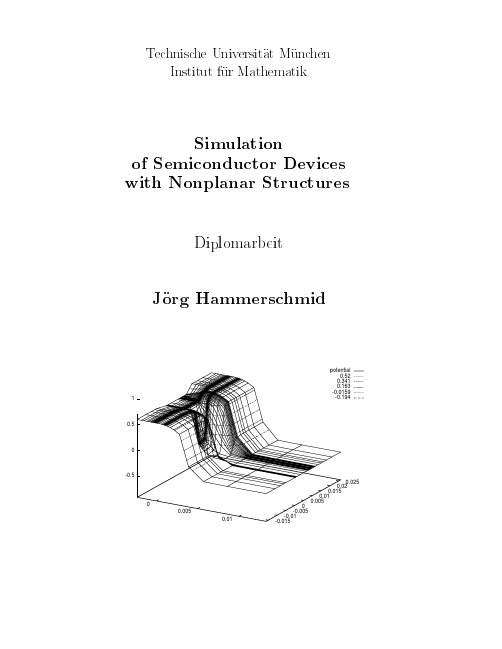
Simulation of Semiconductor Devices with Nonplanar Structures
Diplomarbeit
Jorg Hammerschmid
Aufgabensteller: Prof. Dr. Christoph Zenger Betreuer: Dr. habil. Ulrich Rude Abgabedatum: 15. Mai 1995
1
0.5
0
-0.5 0.025 0.02 0.015 0.01 0.005
0 0.005 0.01
0 -0.005 -0.01 -0.015
Technische Uniathematik
Technische Universitat Munchen Institut fur Mathematik
der klassischen Funf-Punkte-Diskretisierung. Die in dieser Arbeit besprochenen Korrekturtechniken verandern die Diskretisierung von inneren Punkten nicht. Im zweiten Kapitel werden mehrere Ansatze fur eine Korrekturtechnik fur die Poissongleichung gemacht. Bei der bisher verwendeten Diskretisierung wird das Potential zwischen zwei benachbarten Gitterpunkten als linear angenommen. Diese Annahme ist fur Interfacepunkte falsch. Das Potential hat am Interface einen Knick, da die Dielektrizitatskonstante im Halbleiter einen anderen Wert hat als im Isolator. In den ersten drei Losungsansatzen werden die Schnittpunkte zwischen Interface und Gitterlinien als Hilfspunkte eingefuhrt. Das Potential an diesen Schnittpunkten wird dann folgenderma en bestimmt: Durch den Schnittpunkt P 0 wird eine Gerade gelegt, die senkrecht auf dem Interface steht. Diese Gerade wird nach jeder Seite solange verlangert, bis sie auf jeder Seite eine Gitterlinie schneidet. Die Schnittpunkte seien Psem im Halbleiter und Pins im Isolator. Das Potential an diesen zwei Punkten wird mittels linearer Interpolation bestimmt. Mit Hilfe der Interfacebedingung kann jetzt das Potential am Punkt P 0 durch das Potential an diesen zwei Punkten ausgedruckt werden. Fur den ersten und zweiten Losungsansatz wurde die Boxintegrationsmethode als Grundlage gewahlt, fur den dritten Losungsansatz ist der klassische Funf-Punkte-Stern die Grundlage. Die Bestimmung des Potentials am Punkt P 0 mittels der oben beschriebenen Methode macht allerdings Probleme, da nicht berucksichtigt wird, da das Potential an Gitterlinien einen Knick hat. Der vierte Losungsansatz geht davon aus, da das Potential zwischen zwei Gitterpunkten auch dann linear ist, wenn diese zwei Punkte durch das Interface getrennt sind. Als Ausgleich dafur wird die Dielektrizitatskonstante an Interfacepunkten modi ziert. Die Basis fur diese Uberlegungen bildet das physikalische Modell der Kondensatoren. Sind in einem Kondensator zwei Materialien mit unterschiedlicher Dielektrizitatskonstante vorhanden, so la t sich mit Hilfe der Kondensatorgleichung die Dielektrizitatskonstante des gesamten Kondensators bestimmen. Hier wird allerdings vorausgesetzt, da das Interface die Gitterlinien senkrecht schneidet. Mit der Annahme, das das Potential entlang des Interface stuckweise konstant ist, erhalt man ein ahnliches Ergebnis. Als nachstes wird die rechte Seite, passend zu dieser Methode, modi ziert. Dazu wird zunachst das eindimensionale Problem betrachtet und dann auf das zweidimensionale Problem ubertragen. Im eindimensionalen Fall zeigen sich deutliche Vorteile gegenuber der Boxintegrationsmethode. Die Annahme von stuckweise konstantem Potential entlang des Interface fallt hier weg. Zum Schlu ; dieses Kapitels wird der Abbruchfehler der Boxintegrationsmethode mit dem Abbruchfehler des vierten Losungsansatzes verglichen. Unter der Annahme von stuckweise konstantem Potential am Interface, ist die Ordnung des ii

CFD modeling to study fluidized bed combustion and gasication

* Corresponding author. Johan Gadolin Fellow, Process Chemistry Center, Abo Academy University, Abo, Finland. Tel.: þ91 (0)161 2560327; fax: þ91 161 2502240. E-mail address: dr.rjassar@ (R.I. Singh). 1 On EOL (without pay leave) from Department of Mechanical Engineering, Guru Nanak Dev Engineering College, Ludhiana, India. 1359-4311/$ e see front matter Ó 2012 Elsevier Ltd. All rights reserved. /10.1016/j.applthermaleng.2012.12.017
h i g h l i g h t s
< Summary of CFD modeling to study combustion/gasiﬁcation in ﬂuidized bed is done. < Equations for CFD modeling for ﬂuidized bed combustion/gasiﬁcation explained. < CFD modeling can predict heat ﬂux, ﬂow, temperature, ash deposits and emissions. < Trends, challenges and future research areas in this ﬁeld are explored.

1、下载文档前请自行甄别文档内容的完整性，平台不提供额外的编辑、内容补充、找答案等附加服务。
2、"仅部分预览"的文档,不可在线预览部分如存在完整性等问题,可反馈申请退款(可完整预览的文档不适用该条件!)。
3、如文档侵犯您的权益，请联系客服反馈,我们会尽快为您处理(人工客服工作时间：9:00-18:30)。

Proceedings of the 2005 Winter Simulation ConferenceM. E. Kuhl, N. M. Steiger, F. B. Armstrong, and J. A. Joines, eds.ABSTRACTA model of malicious intrusions in infrastructure facilities is developed that uses a network representation of the sys-tem structure together with Markov models of intruder progress and strategy. Simulation is used to analyze vary-ing levels of imperfect information on the part of the in-truders in planning their attacks. This provides an explicit mechanism to estimate the probability of successful breaches of physical security, and to evaluate potential means to reduce that probability.1INTRODUCTIONThere is widespread interest in protection of critical infra-structure from malicious attack. The attacks might be ei-ther physical intrusions (e.g., to steal vital material, plant a bomb, etc.) or cyber intrusions (e.g., to disrupt information systems, steal data, etc.) and the attackers may be interna-tional terrorists, home-grown hackers, or ordinary crimi-nals. In 1997, the report of the U.S. President’s Commis-sion on Critical Infrastructure Protection (PCCIP) identified eight critical infrastructures “whose incapacity or destruction would have a debilitating impact on our de-fense and economic security” (PCCIP 1997). These eight are: telecommunications, electric power systems, natural gas and oil, banking and finance, transportation, water supply systems, government services and emergency ser-vices.In this analysis, we focus primarily on transportation facilities, but the approach we suggest could also be used in other infrastructure contexts. For example, a similar type of analysis has been applied to information systems by Carlson et al. (2004). The objective of the analysis pre-sented here is to provide guidance to system owners and operators regarding effective ways to reduce vulnerabilities of specific facilities. To accomplish this, we develop a Markov Decision model of how an intruder might try to penetrate the various barriers designed to protect the facil-ity. This intruder model provides the basis for considera-tion of possible strategies to reduce the probability of a successful attack on the facility.Our primary attention in this paper is on how varying levels of information about the infrastructure system af-fects the strategies of potential intruders, how the overall probability of intruder success is affected by their level of information, and what implications this has for effective defense of the system against intrusion.We represent the system of interest as a network of nodes and arcs. Nodes represent barriers that an intruder must penetrate, and arcs represent movements between barriers that an intruder can make within the system. Sev-eral previous authors have used graph-based methods to represent attackers or defenders in security analyses. Phil-lips and Swiler (1998) introduced the concept of an “attack graph” to represent sets of system states and paths for an attacker to pursue an objective in disrupting an information system. Several subsequent papers (e.g., Swiler et al. 2001, Jha et al. 2002, Sheyner et al. 2002) have extended these initial ideas.The adversaries first must penetrate entry points to the system, and if an attempted penetration at a particular entry node is successful, they can traverse edges from the suc-cessfully breached node to other nodes in the network that are connected to the one breached. Traversing an edge en-tails a risk of detection. The adversary is assumed to make the decision that maximizes what he/she perceives to be the probability of successful attack. If this perception is in-accurate, the strategy pursued may not be optimal and the overall probability of success is reduced.We can think of this analysis as having three layers. At the bottom layer, the physical characteristics of individual barriers are translated into summary probabilities of detec-tion, success, etc., for use in the middle level model. This middle layer is a Markov Decision Process (MDP) model that represents the optimization of the intruder’s strategy,SIMULATION OF IMPERFECT INFORMATION IN VULNERABILITY MODELING FOR INFRASTRUCTURE FACILITIESDean A. JonesSandia National LaboratoriesPO Box 5800 MS 1138 Albuquerque, NM 87185-1138, U.S.A MarkA.TurnquistLinda K. NozickSchool of Civil & Environmental Engineering309 Hollister HallCornell UniversityIthaca, NY 14850, U.S.A.given the perceived values of detection probabilities, etc. The perceptions may have different levels of accuracy. At this level, we use both simulation and optimization tools. Simulation is used to represent varying perceptions of the system parameters by intruders, and optimization is used to create strategies on the part of intruders, given those per-ceptions. At the top layer of analysis, the system operator (or defender) examines the probabilities of success on the part of potential intruders and the paths that they are likely to follow through the network, and makes changes to re-duce the system vulnerabilities. Those changes may be de-signed either to reduce the real success rates of intruders in penetrating system barriers, or to decrease the accuracy of the information available to the intruders so that their at-tempts to optimize strategies are less effective.At the lowest layer, we use Hidden Markov Models (HMM) to represent an intruder’s actions at a single node (barrier) in a system and the associated “signals” those ac-tions provide that can lead to detection. Then we develop an aggregated representation of that single-node model for inclusion in an MDP model of intruder strategy within a network representation of the entire system at the middle layer. These parts of the analysis are described in detail by Carlson et al. (2004) and Jones et al. (2005). In the inter-ests of space, they will not be included here, so that we may focus this paper on the interaction of simulation and optimization analysis at the middle layer.2MARKOV DECISION MODEL OF INTRUDER STRATEGYAt the system level, we represent a network of barriers and potential movements as shown in the example in Figure 1, representing a simplified hypothetical attempt by an in-truder to place a delayed-action (e.g., altitude detonated) explosive device on an aircraft sitting at a gate in an airport terminal.The intruder must first gain access to the apron area of the terminal. We postulate that this can occur either by gaining illicit access through the employee gate (e.g., by stealing an employee ID and using it to enter the area), or by entering in a service vehicle at a gate (e.g., in a catering truck). If the intruder is successful in getting access to the area, he/she must then impersonate a legitimate worker in the aircraft gate area – either an airline employee or a ser-vice contractor. The “cross-over” arcs between “entry” and “impersonation” in Figure 1 indicate that even if the in-truder gained access to the apron area using an employee ID, he/she may switch ID’s and impersonate a service con-tractor within the area (or vice versa). This impersonation must be successful for the period of time required to get from the entrance to the aircraft itself.Approaching the aircraft carries a risk of detection, and the approachable areas on the aircraft if the intruder is impersonating an employee may be different from those that are approachable if he/she is impersonating a service contractor. For example, a person who appears to be an air-line maintenance employee might not attract attention ap-proaching the under-wing area around the landing gear, whereas a person who appears to be a catering contractor would. For purposes of this example, we consider three ar-eas of the aircraft where an explosive device might be hid-den – inside the wing around the landing gear, in the cargo hold, or in the catering supplies delivered to the galley.If access to the aircraft is gained, the device must be placed without arousing suspicion. This is represented by the arcs connecting the aircraft area nodes to the exit node. Each of these arcs has a probability of detection.Finally, if the intruder succeeds in gaining access to the aircraft and placing the device, he/she must exit with-out detection, and this represents the last barrier. Our mod-eling premise is that if the intruder is detected after placing the device, it will trigger a thorough search of the aircraft and the device will be discovered, so that the attempted at-tack will be foiled.To generalize from this specific example, in a network representing some infrastructure facility or system, if the intruder is successful at breaching a particular barrier, he/she has choices about where to go next (which arc to cross). Crossing arc ij entails a probability of detection, ijδ, and this is represented in the transition matrix.Placement of an Explosive Device on an AircraftIf the intruder is in state i and chooses action a i, we denote the expected value of the future stream of rewards by w(i,ai). Each possible action a i implies a change in the transition probabilities that govern the process. We denote the elements of the transition matrix resulting from choos-ing action a i as P ij(a i). The MDP we define for this prob-lem is positive bounded, and we can find the optimal pol-icy through either policy iteration or linear programming (Puterman 1994).Table 1 summarizes the hypothetical node data used for the example analysis, and Table 2 shows the probabili-ties of detection used for the arcs in the example network. Note that we assume there is no retreat at the stage of exit-ing after placing the device – at that stage either the attackAircraftis successful or it is detected. Also note that the probability of detection on the arcs leading to the “impersonation” nodes is zero. This is because we are treating impersona-tion process (and time) as a barrier (node), so the probabil-ity of detection is lumped at the nodes, rather than on the arcs.Table 1: Example Data for Network NodesNode #NodeDescription(seeFigure 1)ExpectedTime ForAt-temptedBreach(min)Prob.OfSuc-cessProb.ofDetectionProb.ofRe-treat1 EmployeeGate 1 0.20.650.152 ServiceGate2 0.25 0.7 0.053 ImpersonateEmployee10 0.2 0.6 0.24 ImpersonateContractor15 0.4 0.5 0.15 LandingGear5 0.15 0.8 0.056 CargoHold 3 0.1 0.75 0.157 Galley 15 0.150.75 0.18 UndetectedExit10 0.8 0.2 0Table 2: Probability of Detection for Possible MovesArc Prob.ofDetection Empl. Gate – Impersonate Employee 0 Empl. Gate – Impersonate Contractor 0 Service Gate – Impersonate Empl. 0 Service Gate – Impersonate Contr.0 Impersonate Empl. – Landing Gear 0.7Impersonate Empl. – Cargo Hold 0.7Impersonate Contr. – Cargo Hold 0.6Impersonate Contr. – Galley 0.6Landing Gear – Exit 0.4Cargo Hold – Exit 0.2Galley – Exit 0.3 If an intruder knew the structure of the network (Fig-ure 1) and the values in Tables 1 and 2, we would consider him/her to be perfectly informed. Under this assumption, an optimal intrusion strategy (i.e., one that maximizes the probability of successful attack) can be constructed by solving the MDP. For the set of input data in Figure 1 and Tables 1 and 2, the solution for the optimal intruder strat-egy can be summarized as shown in Figure 2. To the left of each node is the probability of successful attack, given that the intruder is “arriving at” that barrier. To the right of each node is the probability of success, given that the in-truder has successfully negotiated that barrier. There is only one value shown for the exit node (i.e., the “approach-ing” probability), because once that node is successfully negotiated, the attack has been a success, by definition.The light colored arcs indicates the optimal path for an intruder (i.e., the path that maximizes the probability of success). This is the path of greatest vulnerability to the system. In our simple example, we would compute a prob-ability of successful attack of 0.0034 for an intruder whose strategy is to gain entry to the apron area through the ser-vice vehicle gate, then impersonate a contractor (probably a catering service worker) to access the aircraft galley and place the device there before exiting.The existence of this strategy does not mean that all intruders will always proceed in exactly the way indicated. It does mean that if an intruder were perfectly informed, this would be a strategy through which the probability of a successful attack could be maximized. In actuality, the probability of successful attack is likely to be less than this maximum value because intruders will have less-than-complete information and may not optimize their strategy. The solution to the MDP also provides useful information on the conditional probability of success for an attacker that reaches a certain point in the network, regardless of whether or not he/she followed the optimal strategy. For example, if an intruder succeeds in reaching the cargo hold of the aircraft (despite the fact that this is not an optimal strategy), the probability of a successful attack from that point on is 0.064.Figure 2: Summary of Intruder Strategy and Probability of Success under Perfect Information3REPRESENTING IMPERFECT INFORMATION One useful representation of imperfect information is to assume that a potential intruder does not know the values of the probabilities in Tables 1 and 2, but has perceptions of those probabilities that contain errors. An intruder with imperfect information will attempt to construct an optimalAircraftstrategy, but because of errors in perception of detection probabilities, the strategy is likely to actually be subopti-mal against the real probabilities. Simulation is an effective tool to explore the effects of imperfect information repre-sented in this way.Suppose that the perception of a given detection prob-ability is represented as a beta random variable with pa-rameters a > 0 and b > 0. The mean of such a random vari-able is b a a +, and the variance is 2))(1(b a b a ab+++. If the intruder’s perception of an unknown probability π is unbiased, π=+ba a, and we can express one of the pa-rameters in terms of the other – e.g., ππab )1(−= . By varying a, we can change the variance (i.e., the level of un-certainty in the perception of π) and set b in terms of a to maintain the same expected value. A convenient way to create experiments is to set the coefficient of variation for the distribution and then solve for the values of a and b that will maintain the desired mean and achieve the required standard deviation. The coefficient of variation for the betadistribution is)1(++b a a b.Alternatively, we can assume that the intruder’s per-ception of the unknown probability may be biased. If we specify both the coefficient of variation in the distributionand the degree of bias (ba a+−π ), we can solve for val-ues of a and b to satisfy those requirements.For any setting of the values for the parameters a and b, we can sample from the perception distribution to simu-late an intruder operating with some specified level of im-perfect information. Of course, this concept extends to im-perfect information with respect to any number of probability estimates. Replicating this simulated sampling leads to varying choices of paths through the network by the imperfectly informed intruder, each of which has a dif-ferent probability of success. This allows construction of an estimated probability distribution for the likelihood of successful attack by an intruder operating at that level of imperfect information, as well as a probability distribution over possible paths through the network. The distribution of path choices allows us to reach some conclusions re-garding the likelihood that an intruder will appear at cer-tain points in the network. 4ILLUSTRATIVE SIMULATION RESULTSTo illustrate these ideas, we will consider a series of ex-periments using the basic network from Figure 1, andcompare the results to the perfect-information solution in Figure 2. As a first experiment we assume that the in-truder’s perception of the detection probabilities (at the nodes and along the arcs) is unbiased, but has a coefficient of variation of 0.1 for all non-zero probabilities (i.e., ex-cluding the first four entries in Table 2).As an example of the beta distribution parameter com-putations, consider the detection probability for the arc connecting “Impersonate Contractor” to “Cargo Hold” (the seventh row of Table 2). The true value for this probability is 0.6. To determine the a and b parameters of the beta dis-tribution to represent imperfect information, we establish the two equations:6.0=+ba a(1)1.0)1(=++b a a b(2)We then solve for a and b, leading to the values a = 39.4 and b = 26.27. This computation is repeated (for dif-ferent underlying probabilities in equation 1) to produce a and b parameters for all the non-zero detection probabili-ties.In each simulation experiment, the success probability for a given node or arc is adjusted to accommodate the sampled value of the detection probability. The retreat probabilities at the nodes are unchanged. This adjustment ensures that the required probabilities sum to 1.0.Table 3 summarizes the results of 30 replications of the simulation. The path descriptors use the node number-ing scheme from Table 1, and are listed in order of de-creasing probability of success. The probabilities of use are rounded to two decimal places, and may not add exactly to 1.0. The path found in the perfect-information case (2-4-7-8) is one of the two most likely paths when the intruder has imperfect information, but approximately 63% of the time, the imperfectly informed intruder will choose a suboptimal path, even when the variability in the perceptions of detec-tion probabilities (as measured by the coefficient of varia-tion) is relatively small (0.1). The average probability of success for an intruder with this level of information is .00279, approximately 17% lower than for the perfect in-formation case. This experiment indicates that even a little reduction in information about the system can have a sig-nificant effect on reducing the likelihood of a successful attack.In addition to information on average probability of success, the path data and probabilities in Table 3 can be used to estimate the likelihood that an intruder will appear at a given point in the network, given the level of imperfect information hypothesized. This is done simply by summing probabilities for paths that include a given node or arc. ForTable 3: Summary of Results When Probability Estimates Are Unbiased and Coefficient of Variation Is 0.1Chosen Path Probabilityof UseProbabilityof Success2-4-7-8 0.37 .003361-4-7-8 0.17 .002692-4-6-8 0.37 .002561-4-6-8 0.07 .002052-3-5-8 0.03 .00108 example, we might be particularly interested in the relative likelihoods of attempts to place explosives in the three dif-ferent areas of the aircraft. In this case, we could use the results in Table 3 to conclude that the probabilities of an intruder attempting to use the landing gear (node 5), the cargo hold (node 6) and the galley (node 7) are .03, .44 and .54, respectively (again rounded to two decimal places).Further insight into the effects of imperfect informa-tion can be obtained by increasing the level of uncertainty.A second experiment increased the coefficient of variation in the detection probability perceptions to 0.3. The percep-tions are still considered to be unbiased. Table 4 summa-rizes the results, again based on 30 replications of the simulation.Table 4: Summary of Results When Probability Estimates Are Unbiased and Coefficient of Variation Is 0.3Chosen Path Probabilityof UseProbabilityof Success2-4-7-8 0.33 .003361-4-7-8 0.23 .002692-4-6-8 0.27 .002561-4-6-8 0.07 .002052-3-5-8 0.03 .001081-3-5-8 0.07 .00086 Comparing Table 4 to Table 3, we see that the increase in uncertainty about the correct detection probabilities causes the optimal path to be chosen less frequently, and a very suboptimal path (1-3-5-8) appears in the list of possi-bilities. Overall, the average probability of success is .00266. This is a decrease from the case where the coeffi-cient of variation is 0.1, but only about 5%. In this sample problem at least, a small amount of uncertainty in the per-ceived detection probabilities is important, but making that uncertainty much larger has relatively little effect on the expected probability of successful attack, as long as the perceptions are unbiased.There is a somewhat more noticeable effect of the in-crease in uncertainty on the probabilities of the intruder at-tempting to use different parts of the aircraft. From the re-sults in Table 4, we can compute estimates of the probability that the intruder would attempt to use the land-ing gear (node 5), the cargo hold (node 6) and the galley (node 7) as 0.1, 0.34, and 0.56, respectively. There is a no-ticeable shift in likelihood from the cargo hold to the land-ing gear for less well-informed intruders. This insight can be helpful to security forces.To test the effects of biased perceptions, we have con-ducted a third simulation experiment. The coefficients of variation in the detection probability perceptions are set to 0.1, as in the first experiment, but we introduce a bias on two of the perceived probabilities – the detection probabili-ties associated with a contractor approaching the aircraft, either the cargo hold or the galley. In Table 2, the “true” values are indicated to be 0.6, but we assume that the in-truder believes (on average) that the values are 0.9 for both probabilities. Intuitively, we expect that these mispercep-tions will tend to drive the intruder’s attack path away from paths that use those two arcs, and since one of the two arcs is part of the optimal path under perfect information, the net effect should be a reduction in success probability for the intruder.Table 5 summarizes the results of the experiment, again based on 30 simulation replications. The overall av-erage probability of success for an attack is reduced to .00144, a reduction of 48% from the value in experiment 1 (.00279), and a reduction of 57% from the original value based on perfect information. The misperception of detec-tion probabilities on the two arcs makes it much less likely that the intruder will attempt to use those arcs (probability of 0.23 versus 0.97 in the first experiment). Attacks are much more likely to be focused on paths (and areas of the aircraft) where the real detection probability is higher, leading to much lower success probability for the intruder. In the results shown in Table 5, the probability of the in-truder attempting to use the landing gear area is 0.37, as compared to 0.03 in experiment 1, and the probability of attempts through the galley has decreased from 0.54 to 0.1. Table 5: Summary of Results When Probability Estimates Are Biased on Arcs 4-6 and 4-7ChosenPathProbabilityof UseProbabilityof Success2-4-7-8 0.10 .003362-4-6-8 0.13 .002562-3-5-8 0.33 .001082-3-6-8 0.33 .000961-3-5-8 0.03 .000861-3-6-8 0.07 .00077 The level of bias in the perceptions of the detection probabilities on arcs 4-6 and 4-7 used in this experiment is substantial, and smaller assumed biases would create less dramatic results. However, we have only introduced the bias on two arcs in the network. More widespread misper-ceptions would be likely in a larger system. This experi-ment does indicate that creating biased perceptions of de-tection probabilities among potential intruders can be very effective in reducing the likelihood of successful attacks by“steering” those attacks into areas where detection really is very likely.There are several means through which a system op-erator might create such misperceptions. Implementing in-expensive, highly visible (though perhaps not really very effective) detection mechanisms might be one means. Sup-plying disinformation about real operations or procedures may be another, although this has obvious drawbacks as well.5EXTENSIONSSeveral possible extensions to this analysis are possible. First, other aspects of imperfect intruder information could be included, such as imperfect knowledge about what bar-riers (nodes) and arcs exist in the system. This type of im-perfect information can be incorporated into the general analysis framework described in this paper.A second useful extension is to consider where im-provements in security (i.e., increases in detection prob-ability) would be most effective against several classes of potential intruders (i.e., intruders with differing levels of information about the system). The analysis of possible in-vestments to improve security is a vital part of the overall approach we have outlined here, and this is an active area of current work.A third useful extension is to create semi-Markov models for the processes of attempted penetration of barri-ers. This would allow more accurate representation of the uncertain time required to penetrate a given barrier, as well as offer the opportunity for time-dependent detection prob-abilities (i.e., the longer an intruder is present at a barrier, the more likely it becomes that he/she will be detected). This extension could improve the range of applicability of the model.6CONCLUSIONSWe have developed a model of intruder actions in attack-ing an infrastructure system based on a Markov Decision Process (MDP). Lower level models of intruder detection at barriers (nodes) of the system can be built as Hidden Markov Models, and the results of those lower level mod-els can be aggregated for use in the MDP of intruder strat-egy for attacking the system. A key aspect of this analysis is representing imperfect information on the part of the in-truders, and this paper focuses on that part of the analysis. Simulation is used as a tool to evaluate the effects of vary-ing levels of imperfect information, sampling from distri-butions of detection probabilities and using those samples to construct distributions of intruder path choices through the network and overall success probability.A small example problem illustrates that even rela-tively small amounts of uncertainty in the information the intruders have about the system can significantly affect the probability that they can mount a successful attack. If the uncertainty is combined with bias in the perceptions of some system parameters, the effect on the intruders is magnified. In the small example studied, biased percep-tions of two key detection probabilities combined with small amounts of uncertainty in perceptions of all the de-tection probabilities reduces the likelihood of a successful attack by a factor of about two. In addition to allowing usto estimate the probability of a successful intrusion, the simulation also allows us to estimate the likelihood of at-tacks appearing at specific locations in the network. This is very useful information for security forces.Several extensions are possible within the frameworkof the model developed here, and efforts to extend and im-prove the analyses are ongoing. This approach appears to offer a significant new tool for evaluating and improvingthe security of infrastructure facilities.REFERENCESCarlson, R., Turnquist, M.A. and Nozick, L.K. 2004. Ex-pected losses, insurability, and vulnerability to attacks,Report SAND2004-0742, Sandia National Laborato-ries, Albuquerque, NM.Jha, S., Sheyner, O., and Wing, J.M. 2002. Minimization and reliability of attack graphs. Research ReportCMU-CS-02-109, School of Computer Science, Car-negie Mellon University, Pittsburgh, PA.http://reports-achive.adm.cs.cmu.edu/anon/2002/CMU-CS-02-109.pdfJones, D.A., Turnquist, M.A. and Nozick, L.K. 2005.Physical security and vulnerability modeling for infra-structure facilities, Working Paper, Sandia NationalLaboratories, Albuquerque, NM.Phillips, C.A., and Swiler, L.P. 1998. A graph-based Sys-tem for network-vulnerability analysis, In ACM Pro-ceedings for the 1998 New Security Paradigms Work-shop, pp. 71-81.Puterman, M.L. 1994. Markov decision processes. Wiley, New York.President’s Commission on Critical Infrastructure Protec-tion 1997. Critical foundations: Protecting America’sinfrastructures, available on line at .Swiler, L.P., Phillips, C.A., Ellis, D., and Chakerian, S.2001. Computer-attack graph generation tool, Pro-ceedings of the 2nd DARPA Information SurvivabilityConference and Exposition, Vol. 2, pp. 307-321. Sheyner, O., Haines, J., Jha, S., Lippmann, R., and Wing, J.M. 2002. Automated generation and analysis of at-tack graphs,” Proceedings of the IEEE Computer So-ciety Symposium on Research in Security and Privacy,Berkeley, CA, pp. 273-284.。