运筹学ch16
运筹学教程(第三版)习题答案(第一章)

( 3)
max Z = x1 + x 2 6 x1 + 10 x 2 ≤ 120 st . 5 ≤ x1 ≤ 10 5≤ x ≤8 2
( 4)
page 2 3 May 2011
运筹学教程
第一章习题解答
(1) min Z = 2 x1 + 3 x 2 4 x1 + 6 x 2 ≥ 6 st . 2 x1 + 2 x 2 ≥ 4 x ,x ≥ 0 1 2 1 , Z = 3是一个最优解 3
min st x 1 Z = 2 x1 − 2 x 2 + 3 x 3 − x1 + x 2 + x 3 = 4 − 2 x1 + x 2 − x 3 ≤ 6 ≤ 0 , x 2 ≥ 0 , x 3 无约束
(1)
()
page 5 3 May 2011
School of Management
(1)
(2)
page 8 3 May 2011
运筹学教程
第一章习题解答
(1) max Z = 3 x1 + x 2 + 2 x 3 12 x1 + 3 x 2 + 6 x 3 + 3 x 4 = 9 8 x + x − 4 x + 2 x = 10 1 2 3 5 st 3 x1 − x 6 = 0 x j ≥ 0( j = 1, L , 6) ,
运筹学教程(第二版) 运筹学教程(第二版) 习题解答
安徽大学管理学院
洪 文
电话: 电话:5108157(H),5107443(O) , E-mail: Hongwen9509_cn@
(完整版)运筹学》习题答案运筹学答案

《运筹学》习题答案一、单选题1.用动态规划求解工程线路问题时,什么样的网络问题可以转化为定步数问题求解()BA.任意网络B.无回路有向网络C.混合网络D.容量网络2.通过什么方法或者技巧可以把工程线路问题转化为动态规划问题?()BA.非线性问题的线性化技巧B.静态问题的动态处理C.引入虚拟产地或者销地D.引入人工变量3.静态问题的动态处理最常用的方法是?BA.非线性问题的线性化技巧B.人为的引入时段C.引入虚拟产地或者销地D.网络建模4.串联系统可靠性问题动态规划模型的特点是()DA.状态变量的选取B.决策变量的选取C.有虚拟产地或者销地D.目标函数取乘积形式5.在网络计划技术中,进行时间与成本优化时,一般地说,随着施工周期的缩短,直接费用是( )。
CA.降低的B.不增不减的C.增加的D.难以估计的6.最小枝权树算法是从已接接点出发,把( )的接点连接上CA.最远B.较远C.最近D.较近7.在箭线式网络固中,( )的说法是错误的。
DA.结点不占用时间也不消耗资源B.结点表示前接活动的完成和后续活动的开始C.箭线代表活动D.结点的最早出现时间和最迟出现时间是同一个时间8.如图所示,在锅炉房与各车间之间铺设暖气管最小的管道总长度是( )。
CA.1200B.1400C.1300D.17009.在求最短路线问题中,已知起点到A,B,C三相邻结点的距离分别为15km,20km,25km,则()。
DA.最短路线—定通过A点B.最短路线一定通过B点C.最短路线一定通过C点D.不能判断最短路线通过哪一点10.在一棵树中,如果在某两点间加上条边,则图一定( )AA.存在一个圈B.存在两个圈C.存在三个圈D.不含圈11.网络图关键线路的长度( )工程完工期。
CA.大于B.小于C.等于D.不一定等于12.在计算最大流量时,我们选中的每一条路线( )。
CA.一定是一条最短的路线B.一定不是一条最短的路线C.是使某一条支线流量饱和的路线D.是任一条支路流量都不饱和的路线13.从甲市到乙市之间有—公路网络,为了尽快从甲市驱车赶到乙市,应借用()CA.树的逐步生成法B.求最小技校树法C.求最短路线法D.求最大流量法14.为了在各住宅之间安装一个供水管道.若要求用材料最省,则应使用( )。
运筹学实用教程部分作业答案
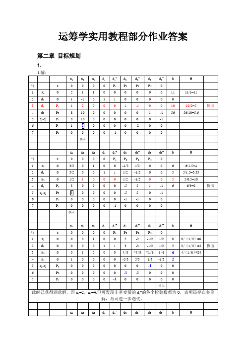
运筹学实用教程部分作业答案第二章目标规划1.2.2. 解:根据题意,设车间每日生产A、B两种产品的数量分别为x1,x2,可得该题目标规划模型:目标规划模型Min Z =P1d1- + P2(d2+ + d3+ + d4+)30x1 + 12x2 + d1-- d1+ =2500 ①2x1 + x2 + d2-- d2+=140 ②s.t.x1 + d3-- d3+=60 ③x2 + d4-- d4+=100 ④x1,x2 ≥0, d i- ,d i+≥0,i=1,2,3,4 ⑤3.3.解:根据题意,设一车间每月生产A、B两种产品的数量分别为x1A.,x1B,二车间每月生产A、B两种产品的数量分别为x2A.,x2B,可得该题目标规划模型:Min Z =P1d1+ + P2(d2-+ d2+)+ P2(d3- + d3+)+ P3(4d4-+ d5-)+ P4d41+50(x1A +x2A)+ 30(x1B +x2B)+ d1-- d1+ =4600 ①x1A +x2A + d2-- d2+=50 ②x1B +x2B + d3-- d3+=80 ③s.t.2x1A + x1B + d4-- d4+=110 ④x 2A + 3x 2B + d 5-- d 5+=150⑤ d 4+ + d 41-- d 41+=20⑥x 1A ,x 2A ,x 1B ,x 2B ≥0, d i -,d i +≥0,i=1,2,3,4,5⑦4.4.解:要建立目标规划模型,题设的条件不够。
第三章 动态规划1.1. 计算下图所示的从A 到E 的最短路线及其长度。
解:略22.解:1.按动态规划要求确定相关参数:(1)将分配问题按零售店1、2、3、4顺序分成四个阶段;(2)各阶段的状态变量S k 取为在各阶段可能分配货物的总箱数,或者说,S k 是分配给第K 个零售店以后(含第K 个零售店)各零售店货物的总箱数; (3)u k 是分配给第K 个零售店的货物箱数; (4)状态转移方程 S k+1= S k - u k (S k )(5)最优指标函数f k (S k )是从第K 阶段开始到最后阶段为止的最大利润:{})(),(max )(11+++=K K K K K u K K S f u S d S f K0)(5=K S f2.下面进行分阶段的计算: 当K=4时,S 4=(0,1,2,3,4,5,6)S 4取不同的值时,f 4(S 4)的计算如下表:第四阶段计算表当K=3时,是将S 3=(0,1,2,3,4,5,6)箱货物分配给3、4两个零售店。
运筹学知识点
运筹学知识点:绪论1.运筹学的起源2.运筹学的特点第一章线性规划及单纯形法1.规划问题指生产和经营管理中如何合理安排,使人力、物力等各种资源得到充分利用,获得最大效益。
2.规划问题解决两类问题:一是给定一定数量的人力、物力等资源,研究如何充分利用,以发挥其最大效果;二是已给定计划任务,研究如何统筹安排,用最少的人力和物力去完成。
3.规划问题的数学模型包含三个组成要素:决策变量、目标函数(单一)、约束条件(多个)。
线性规划问题的数学模型要求:决策变量为可控的连续变量,目标函数和约束条件都是线性的。
4.线性规划问题的标准形式:目标函数为极大、约束条件为等式、决策变量为非负、变量为非负5.划标准型时添加的松驰变量、剩余变量和人工变量6.理解可行解、最优解、基、基解、基可行解等概念,且掌握各类解间的关系7.用图解法理解线性规划问题的四种解的情况:无穷多最优解、无界解、无可行解、唯一最优解8.用图解法只有解决两个变量的决策问题9.线性规划问题存在可行解,则可行域是凸集。
10.线性规划问题的基可行解对应线性规划问题可行域的顶点。
11.线性规划问题的解进行最优性检验:当所有的检验数小于等于零时为最优解;尤其当检验数小于零时(即不等于零)有唯一最优解;当某个非基变量检验数为时,有无穷多最优解;当存在某个检验数大于零且对应的系数又小于等于零时,有无界解。
12.单纯形法的计算过程,可能出计算题13.入单纯形表前首先要化成标准形式。
14.确定换出变量时根据θ值最小原则,且要求公式中对应的系数大于零。
15.当线性规划中约束条件为等式或大于等于时,划为标准型后,系数矩阵中又不包含单位矩阵时,需要添加人工变量构造一个单位矩阵作为基。
16.人工变量的系数为足够大的一个负值,用—M代表17.一般线性规划问题的数学建模题(生产计划问题、人才资源分配问题、混合配料问题等)第二章对偶问题1.原问题和对偶问题数学模型的对应关系,可能出填空题和数学模型题2.每一个线性规划必然有与之相伴而生的对偶问题3.对偶问题的性质:弱对偶性、无界性、强对偶性、最优性、互补松弛性,其中互补松弛性可能出计算题4.原问题与其对偶问题之间存在一对互补的基解,其中原问题的松弛变量对应对偶问题的变量,对偶问题的剩余变量对应原问题变量5.影子价格的定义,用互补松驰性理解影子价格的含义6.影子价格与企业的生产任务、产品结构、技术状况等相关,与市场需求无关7.理解影子价格是机会成本第三章运输问题1.运输问题的数学模型,出建模题2.掌握三个数字:m+n、m*n、m+n-13.解的退化及处理4.运输规划问题本质仍然是线性规划,系数矩阵的特殊性,利用表上作业法求解,核心依然是单纯形法5.表上作业法的计算过程,可能出大题6.什么是基格和空格及含义以及检验数的经济意义7.初始方案的方法,计算检验数的方法,调整方案的方法8.检验数的含义及检验规划与一般线性规划问题的差别9.产销不平衡问题的处理,包括产大于销和销大于产,假想地的单位运价设为零第四章整数规划1.整数规划的分类:纯整数、混合整数、0-1整数2.指派问题的数学模型,可能出建模题3.匈牙利法的计算过程4.解矩阵的特点:n个解1位于不同行不同列上5.分枝定界法分枝和定界的依据以及如何分枝和如何定界6.整数规划问题的求解方法及适用条件7.整数规划问题与其松弛问题解的关系第五章目标规划1.线性规划的局限:严格约束、单目标、约束同等重要2.目标规划问题的数学模型,可能会出建模题,强调目标函数由偏差变量、优先因素和权系数构成3.偏差变量的含义及特点,成对出现,非负且至少有一个为零4.目标约束是等式,等式左边添加一对偏差变量相减5.目标规划问题求解的单纯形表计算停止的规划:要么所有行的检验数均为非负,要么前i行检验数为非负,第i+1行存在负的检验数,但在负检验数上面存在正检验数6.目标规划的达成函数中的偏差变量的选择第六章图论与网络优化1.图论中的图研究对象间的关系,只关心图中有多少个点及点间有线相连2.树的定义及性质3.最小树的求解方法:避圈法和破圈法4.狄克斯屈拉算法的特点:不仅求出从始点到终点的最短路,还求出从始点其他任何各点的最短路5.有向图(点弧)非对称关系和无向图(点边)对称关系的应用6.可行流的定义:两大类的三个条件7.增广链的定义及特点8.最大流最小割定理9.用ford-fulkerson算法求网络中的最大流的计算过程10.算法的核心和实质是判断是否存在增广链,,即网络达到最大流的条件是网络中不存在增广链第七章网络计划技术1.关键路线的定点:持续时间最长、节点时差为零、不止一条2.工作持续时间的确定方法及使用条件3.节点最早时间、节点最迟时间的理解4.工作时间参数着重理解总时差和自由时差,即总时差是若干项工作共同拥有的机动时间,自由时差是某项工作单独拥有的机动时间5.绘制网络技术图的规则第八章动态规划1.动态规划是研究多阶段决策问题的理论和方法2.状态必须具备无后效性,及无后效性的定义3.动态规划和顺序解法和逆序解法的路径及应用条件。
运筹学课后习题答案
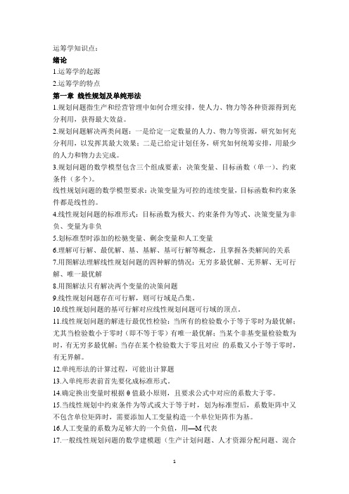
第一章 线性规划1、由图可得:最优解为2、用图解法求解线性规划: Min z=2x 1+x 2⎪⎪⎩⎪⎪⎨⎧≥≤≤≥+≤+-01058244212121x x x x x x解:由图可得:最优解x=1.6,y=6.4Max z=5x 1+6x 2⎪⎩⎪⎨⎧≥≤+-≥-0,23222212121x x x x x x解:由图可得:最优解Max z=5x 1+6x 2, Max z= +∞Maxz = 2x 1 +x 2⎪⎪⎩⎪⎪⎨⎧≥≤+≤+≤0,5242261552121211x x x x x x x由图可得:最大值⎪⎩⎪⎨⎧==+35121x x x , 所以⎪⎩⎪⎨⎧==2321x xmax Z = 8.1212125.max 23284164120,1,2maxZ .jZ x x x x x x x j =+⎧+≤⎪≤⎪⎨≤⎪⎪≥=⎩如图所示,在(4,2)这一点达到最大值为26将线性规划模型化成标准形式:Min z=x 1-2x 2+3x 3⎪⎪⎩⎪⎪⎨⎧≥≥-=++-≥+-≤++无约束321321321321,0,052327x x x x x x x x x x x x解:令Z ’=-Z,引进松弛变量x 4≥0,引入剩余变量x 5≥0,并令x 3=x 3’-x 3’’,其中x 3’≥0,x 3’’≥0Max z ’=-x 1+2x 2-3x 3’+3x 3’’⎪⎪⎩⎪⎪⎨⎧≥≥≥≥≥≥-=++-=--+-=+-++0,0,0'',0',0,05232'''7'''5433213215332143321x x x x x x x x x x x x x x x x x x x7将线性规划模型化为标准形式Min Z =x 1+2x 2+3x 3⎪⎪⎩⎪⎪⎨⎧≥≤-=--≥++-≤++无约束,321321321321,00632442392-x x x x x x x x x x x x解:令Z ’ = -z ,引进松弛变量x 4≥0,引进剩余变量x 5≥0,得到一下等价的标准形式。
运筹学ch.ppt

2z x2 3 x1 3 表示一簇平行线
目标值在(4,2)点,达到最大值14
Prepared by Dr. Jian-Jun Wang 2008
第1章 线性规划与单纯形法 15 / 168
1.2 图解法
《Operations Research》 2019/12/27
a11x1 a12 x2 a1n xn b1
约束条件:a21x1
a22
x2
a2n xn
b2
am1x1 am2 x2 amn xn bn x1,x2 ,,xn 0
Prepared by Dr. Jian-Jun Wang 2008
第1章 线性规划与单纯形法 22 / 168
《Operations Research》 2019/12/27
1.3 线性规划问题的标准型式
用矩阵形式表示的标准形式线性规划
M
'' 1
:目标函数:max
z
CX
约束条件: XAX
0
b
系数矩阵:A
a11
a1n
P1 ,P2
Prepared by Dr. Jian-Jun Wang 2008
第1章 线性规划与单纯形法 4 / 168
1.1 问题的提出
《Operations Research》 2019/12/27
1.1 问题的提出
例 1 某工厂在计划期内要安排生产Ⅰ、Ⅱ两种产品, 已知生产单位产品所需的设备台时及A、B两种原材料 的消耗,如表1-1所示。
, Pn
运筹学完整版
绪论
20世纪50年代中期,钱学森、许国志等教授在国内全面介绍 和推广运筹学知识,1956年,中国科学院成立第一个运筹学研究 室,1957年运筹学运用到建筑和纺织业中,1958年提出了图上作 业法,山东大学的管梅谷教授提出了“中国邮递员问题”,1970 年,在华罗庚教授的直接指导下,在全国范围内推广统筹方法和 优选法。
另外,还应用于设备维修、更新和可靠性分析,项目的选择 与评价,工程优化设计等。
“管理运筹学”软件介绍
“管理运筹学”2.0版包括:线性规划、运输问题、整数规划(0-1整数 规划、纯整数规划和混合整数规划)、目标规划、对策论、最短路径、 最小生成树、最大流量、最小费用最大流、关键路径、存储论、排队论、 决策分析、预测问题和层次分析法,共15个子模块。
x
va2x2x a dv 0 dx
2 ( a 2 x )x ( 2 ) ( a 2 x )2 0
x a 6
线性规划问题的数学模型
例1.2 某厂生产两种产品, 下表给出了单位产品所需资 源及单位产品利润
项目
Ⅰ
设备 A(h) 0
设备 B(h) 6
调试工序(h) 1
利润(元) 2
Ⅱ 每天可用能力
5
经济管理学核心课程
运筹学
( Operations Research )
第一章
运
决
筹
胜
帷
绪论
千
幄
里
之n
外
绪论
本章主要内容: (1)运筹学简述 (2)运筹学的主要内容 (3)本课程的教材及参考书 (4)本课程的特点和要求 (5)本课程授课方式与考核 (6)运筹学在经济管理中的应用
绪论
什么是运筹学? Operational Research 运用研究、 运作研究
运筹学部分课后习题解答
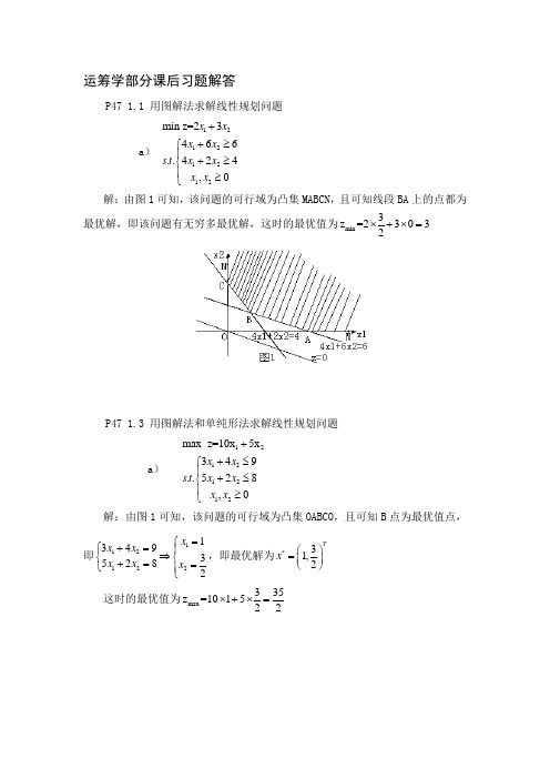
运筹学部分课后习题解答P47 1.1 用图解法求解线性规划问题a)12121212min z=23466 ..424,0x xx xs t x xx x++≥⎧⎪+≥⎨⎪≥⎩解:由图1可知,该问题的可行域为凸集MABCN,且可知线段BA上的点都为最优解,即该问题有无穷多最优解,这时的最优值为min 3z=23032⨯+⨯= P47 1.3 用图解法和单纯形法求解线性规划问题a)12121212max z=10x5x349 ..528,0x xs t x xx x++≤⎧⎪+≤⎨⎪≥⎩解:由图1可知,该问题的可行域为凸集OABCO,且可知B点为最优值点,即112122134935282xx xx x x=⎧+=⎧⎪⇒⎨⎨+==⎩⎪⎩,即最优解为*31,2Tx⎛⎫= ⎪⎝⎭这时的最优值为max335z=101522⨯+⨯=单纯形法: 原问题化成标准型为121231241234max z=10x 5x 349..528,,,0x x x s t x x x x x x x +++=⎧⎪++=⎨⎪≥⎩ j c →10 5B CB Xb 1x2x3x4x0 3x 9 3 4 1 0 04x8[5] 2 0 1 j j C Z -105 0 0 0 3x 21/5 0 [14/5] 1 -3/5 101x8/51 2/5 0 1/5 j j C Z -1 0 -2 5 2x 3/2 0 1 5/14 -3/14 101x11 0 -1/72/7j j C Z --5/14 -25/14所以有*max 33351,,1015222Tx z ⎛⎫==⨯+⨯= ⎪⎝⎭P78 2.4 已知线性规划问题:1234124122341231234max24382669,,,0z x x x x x x x x x x x x x x x x x x x =+++++≤⎧⎪+≤⎪⎪++≤⎨⎪++≤⎪≥⎪⎩求: (1) 写出其对偶问题;(2)已知原问题最优解为)0,4,2,2(*=X ,试根据对偶理论,直接求出对偶问题的最优解。
管理运筹学第16章决策分析

管理运筹学第16章决策分析
§2 风险型情况下的决策
三、决策树法 具体步骤: (1) 从左向右绘制决策树; (2) 从右向左计算各方案的期望值,并将结果标在相应 方案节点的上方; (3) 选收益期望值最大(损失期望值最小)的方案为最优 方案,并在其它方案分支上打∥记号。
EVWPI = 0.3*30 + 0.7*5 = 12.5万 那么, EVPI = EVWPI - EVW0PI = 12.5 - 6.5 = 6万 即这个全情报价值为6万。当获得这个全情报需要的成本小于6 万时,决策者应该对取得全情报投资,否则不应投资。
注:一般“全”情报仍然存在可靠性问题。
管理运筹学第16章决策分析
种, I1 :需求量大; I2 :需求量小。并 且根据该咨询公司积累的资料统计得知,
情况有两种可能发生的自然状态。N1 : 需求量大; N2 :需求量小,且N1的发
当市场需求量已知时,咨询公司调查结 论的条件概率如下表所示:
生概率即P(N1)=0.3; N2的发生概率即
条
自
P(N2)=0.7 。经估计,采用某一行动方
效益(函数)值:v = ( si, nj )
自然状态发生的概率P=P(sj) j =1, 2, 决策模型的基本结构:(A, N, P, V)
…, m
基本结构(A, N, P, V)常用决策表、决策树等表示。
管理运筹学第16章决策分析
§1 不确定情况下的决策
特征:1、自然状态已知;2、各方案在不同自然状态下的收益 值已知;3、自然状态发生不确定。
§2 风险型情况下的决策
首先,由全概率公式求得联合概率表:
运筹学专题知识

2024/10/29
(二)运筹学旳产生
运筹学是一门利用科学,它本身是在利用中产生与发 展旳,产生旳背景为第二次世界大战。
1.“OR”一词旳提出 2.不列颠之战 3.盟军封锁直布罗陀海峡
2024/10/29
一、运筹学旳历史
运筹学旳精粹可归纳为“优化决策”,而优化决策 古已经有之,作为完整、系统旳学科,运筹学产生于本 世纪,古代旳优化决策与当代运筹学旳产生有着旳主动 影响。
(一)朴素旳优化思想
1.赛马与桂陵之战 2.晋国公重建皇城
2024/10/29
1.赛马与桂陵之战
“田忌赛马”是家喻户晓旳历史故事。战国时齐威王与齐相田忌 赛马,双方各出三匹马比赛,每胜一场赢得一千金。因为王府旳 马比相府旳马好,所以田忌每天都要输掉三千金。
巡查机中队击沉击伤德军潜艇3艘,自己无一伤亡。
2024/10/29
(三)运筹学旳发展
战后OR技术被广泛用于经济领域,并得到了很大旳发展。它旳发展大致可 分三个阶段:
1.从1945年到50年代初,被称为创建时期。此阶段旳特点是从事运筹学研 究旳人数不多,范围较小,运筹学旳出版物、研究组织等寥寥无几
2.从50年代早期到50年代末期,被以为是运筹学旳成长时期。此阶段旳一 种特点是电子计算机技术旳迅速发展,使得运筹学中某些措施如单纯形法、动 态规划措施等,得以用来处理实际管理系统中旳优化问题,增进了运筹学旳推 广应用。
2024/10/29
2.晋国公重建皇城
距今约1023年前,开封一场 大火,北宋皇城毁于一旦。宋真 宗命晋国公丁渭,主持重建全部 宫室殿宇。
运筹学习题答案(第一章)

c
x1
j
1
1 0
0 0
-2/14 10/35 -5/14d+2/14c 3/14d-10/14c
School of Management
page 13 15 June 2013
运筹学教程
第一章习题解答
当c/d在3/10到5/2之间时最优解为图中的A点;当 c/d大于5/2且c大于等于0时最优解为图中的B点;当c/d 小于3/10且d大于0时最优解为图中的C点;当c/d大于 5/2且c小于等于0时或当c/d小于3/10且d小于0时最优解 为图中的原点。
x1 0 0 0
x2 3 0 0
基可行解 x3 x4 x5 0 0 3.5 1.5 0 0 3 8 5
x6 0 0 0
Z 3 3 0
0.75
page 9 15 June 2013
0
0
0
2
2.25
2.25
School of Management
运筹学教程
第一章习题解答
min Z 5 x 1 2 x 2 3 x 3 2 x 4 (2) x1 2 x 2 3 x 3 4 x 4 7 st 2 x 1 2 x 2 x 3 2 x 4 3 x j 0 , ( j 1, 4 )
该题是无穷多最优解。 最优解之一: x1 9 5 , x2 4 5 , x3 0, Z 6
page 19 15 June 2013
School of Management
运筹学教程
第一章习题解答
max Z 4 x 1 x 2 3 x1 x 2 3 4 x1 3 x 2 x 3 6 st x 2 x2 x4 4 1 x j 0( j 1, , 4) ,
运筹学课后答案大全
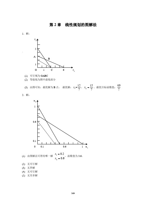
第2章 线性规划的图解法1.解:x`A 1 (1) 可行域为OABC(2) 等值线为图中虚线部分(3) 由图可知,最优解为B 点, 最优解:1x =712,7152=x 。
最优目标函数值:7692.解: x 2 10 1(1) 由图解法可得有唯一解 6.02.021==x x ,函数值为3.6。
(2) 无可行解 (3) 无界解 (4) 无可行解 (5)无穷多解(6) 有唯一解 3832021==x x ,函数值为392。
3.解:(1). 标准形式:3212100023m ax s s s x x f ++++=,,,,9221323302932121321221121≥=++=++=++s s s x x s x x s x x s x x(2). 标准形式:21210064m in s s x x f +++=,,,46710263212121221121≥=-=++=--s s x x x x s x x s x x(3). 标准形式:21''2'2'10022m in s s x x x f +++-=,,,,30223505527055321''2'2'12''2'2'1''2'2'11''2'21≥=--+=+-=+-+-s s x x x s x x x x x x s x x x4.解:标准形式:212100510m ax s s x x z +++=,,,8259432121221121≥=++=++s s x x s x x s x x松弛变量(0,0) 最优解为 1x =1,x 2=3/2.标准形式:32121000811m in s s s x x f ++++=,,,,369418332021032121321221121≥=-+=-+=-+s s s x x s x x s x x s x x剩余变量(0.0.13) 最优解为 x 1=1,x 2=5.6.解:(1) 最优解为 x 1=3,x 2=7. (2) 311<<c (3) 622<<c (4)4621==x x(5) 最优解为 x 1=8,x 2=0. (6) 不变化。
运筹学(第三章)课件

i =1
例1:
某市有三个造纸厂A1,A2和A3,其纸的产量分别为 8,5和9个单位。由各造纸厂到各用户的单位运价 如表所示,请确定总运费最少的调运方案。
销地 产地 A1
A2
A3 销量
B1 3 11 6
4
B2 12 2 7
3
B3 3 5 1
5
B4
产量
4 8
9 5
5 9
6
运筹学(第三章)
销地 产地 A1
A2
A3 销量
B1 4
8
2
8
8
B2
12
8
10
6
5
14
B3
4
3
4
11
8
12
B4
产量
11
16 ②
9
10 ④
6
14
22 ⑥
14
48
①
③
⑤
⑥
8×4+8×12 +6×10+4×3+8×11+14×6= 372(元)
运筹学(第三章)
最小元素法——每次找最小元素
销地 产地 A1
A2
A3 销量
B1 4
2
8
8
8
B2 12
价为 cij (i = 1,2,..., m; n = 1,2,..., n) ,又假设产销是平衡的,即:
m
n
ai = b j ,问应如何安排运输可使总运费最小?
i =1
j =1
运筹学(第三章)
二、运输问题的数学模型
假定 xij 表示由 Ai 到 B j 的运输量,则平衡条件下的运输问题可写出
用表上作业法求解运输问题
运筹学知识点总结
运筹学:应用分析、试验、量化的方法,对经济管理系统中人力、物力、财力等资源进行统筹安排,为决策者提供有依据的最优方案,以实现最有效的管理。
第一章、线性规划的图解法1.基本概念线性规划:是一种解决在线性约束条件下追求最大或最小的线性目标函数的方法。
线性规划的三要素:变量或决策变量、目标函数、约束条件。
目标函数:是变量的线性函数。
约束条件:变量的线性等式或不等式。
可行解:满足所有约束条件的解称为该线性规划的可行解。
可行域:可行解的集合称为可行域。
最优解:使得目标函数值最大的可行解称为该线性规划的最优解。
唯一最优解、无穷最优解、无界解(可行域无界)或无可行解(可行域为空域)。
凸集:要求集合中任意两点的连线段落在这个集合中。
等值线:目标函数z,对于z的某一取值所得的直线上的每一点都具有相同的目标函数值,故称之为等值线。
松弛变量:对于“≤”约束条件,可增加一些代表没使用的资源或能力的变量,称之为松弛变量。
剩余变量:对于“≥”约束条件,可增加一些代表最低限约束的超过量的变量,称之为剩余变量。
2.线性规划的标准形式约束条件为等式(=)约束条件的常数项非负(b j≥0)决策变量非负(x j≥0)3.灵敏度分析:是在建立数学模型和求得最优解之后,研究线性规划的一些系数的变化对最优解产生什么影响。
4.目标函数中的系数c i的灵敏度分析目标函数的斜率在形成最优解顶点的两条直线的斜率之间变化时,最优解不变。
5.约束条件中常数项b i的灵敏度分析对偶价格:约束条件常数项中增加一个单位而使最优目标函数值得到改进的数量。
当某约束条件中的松弛变量(或剩余变量)不为零时,这个约束条件的对偶价格为零。
第二章、线性规划问题在工商管理中的应用1.人力资源分配问题(P41)设x i为第i班次开始上班的人数。
2.生产计划问题(P44)3.套材下料问题(P48)下料方案表(P48)设x i为按各下料方式下料的原材料数量。
4.配料问题(P49)设x ij为第i种产品需要第j种原料的量。
运筹学16
Chap16 Markov ChainsWe often are faced with making decision based upon phenomena that have uncertainty associated with them. Their variation can be described by aprobability model.9We present probability models for processes that evolve over time in a probabilistic manner. Such processes are called stochastic processes.A stochastic process is defined to be an indexed collection of random variables{X t}, where the index t runs through a given set T.9X t represents a measurable characteristic of interest at time t.9Example: {X0, X1, X2, …} represent the collection of weekly inventory of a product.A general structure of a stochastic process9At particular points of time t labeled 0, 1, …, the system is found in exactly one of a finite number of mutually exclusive categories or states labeled 0, 1, …, M.There are M+1 states totally.9Thus, the stochastic process {X t} = {X0, X1, X2, …} provides a mathematical representation of how the status of the physical system evolves over time.9This kind of process is referred to as being a discrete time stochastic process with a finite state space.A Weather Example9The probability of being dry tomorrow is 0.8 if it is dry today, but is only 0.6 if it rains today.9These probabilities do not change if information about the weather before today is also taken into account.9The evolution of the weather from day to day is a stochastic process.9Starting on some initial day (labeled as day 0), the weather is observed on each day t, for t = 0, 1, 2, …. The state of the system on day t can be either State 0(day t is dry) or State 1 (day t has rain).9Thus, the random variable X t = 0, if day t is dry; and X t = 1, if day t has rain.An Inventory Example9A store stocks a particular model camera that can be ordered weekly.9Random variables D1, D2,…, D t represent the demand for this camera during the t th week (number of cameras that would be sold in week t if the inventory is not depleted).¾Assume that the D t are independent and identically distributed random variable having a Poisson distribution with a mean of 1.9Let X0 represent the number of cameras on hand at the outset, X t (t = 1, 2, …) the number of cameras on hand at the end of week t.9{X t } = {X0, X1, X2, …} is a stochastic process where the random variable X t represents the state of the system at time t.9Assume X0 is 3, so that week 1 begins with three cameras on hand.9Order is placed at the end of each week t with the following policy: ¾If X t = 0, order 3 cameras.¾If X t > 0, do not order any camera.9Thus, X t+1 = max{3 – D t+1, 0}, if X t = 0;X t+1 = max{X t – D t+1, 0}, if X t≥1.9The possible states are 0, 1, 2, and 3.Markov Chain9A stochastic process {X t} is said to have the Markovian property ifP{X t+1 = j | X0 = k0, X1 = k1, …, X t-1 = k t-1, X t = i} = P{X t+1 = j | X t = i},for t = 0, 1, … and every sequence i, j, k0, k1, …, k t-1.9That is, the conditional probability of any future event depends only upon the present state.9A stochastic process {X t } (t = 0, 1, …) is a Markov chain if it has the Markovian property.9The conditional probabilities P{X t+1 = j | X t = i} are called (one-step) transition probabilities.9If, for each i and j, P{X t+1 = j | X t = i} = P{X1 = j | X0 = i} for all t = 0, 1…., then the (one-step) transition probabilities are said to be stationary and are denoted by p ij.¾The stationary transition probability implies that the transition probabilities do not change over time.9The stationary transition (one-step) probabilities implies that P{X t+n = j | X t = i} = P{X n= j | X0 = i} for each i, j, and n (n = 0, 1, 2, …). Usually, denote as n-step transition probabilities p ij(n).¾ When n = 1, p ij (1) = p ij . ¾ p ij (n ) ≥ 0. ¾10)(=∑=Mj n ij p for all i ; n = 0, 1, 2, ….¾ A convenient notation for representing the n -step transition probabilities isP (n )= ⎥⎥⎥⎥⎥⎦⎤⎢⎢⎢⎢⎢⎣⎡)()(1)(0)(1)(11)(10)(0)(01)(00.....................n MM n M n M n M n n n M n n p p p p p p p P p ¾ We drop the superscript n when n = 1 and refer to this as the transitionmatrix .P = ⎥⎥⎥⎥⎥⎦⎤⎢⎢⎢⎢⎢⎣⎡MM M M M M p p p p p p p P p .................. (1011110)00100 Formulating the Weather Example as a Markov Chain9 Recall that P {X t +1 = 0 | X t = 0} = 0.8 and P {X t +1 = 0 | X t = 1} = 0.6.9 These probabilities do not change if information about the weather before today(day t ) is also taken into account. P {X t +1 = 0 | X 0 = k 0, X 1 = k 1, …, X t -1 = k t -1, X t = 0} = P {X t +1 = 0 | X t = 0} P {X t +1 = 0 | X 0 = k 0, X 1 = k 1, …, X t -1 = k t -1, X t = 1} = P {X t +1 = 0 | X t = 1} (Also hold if X t +1 = 0 is replaced by X t +1 = 1.)9 This stochastic process has the Markovian property; so the process is a Markov chain. 9 Thus, the transition matrix isP =Formulating the Inventory Example as a Markov Chain9 X t is the number of cameras in stock at the end of week t is a Markov chain.9 Need to obtain the (one-step) transition probabilities P = ⎥⎥⎥⎥⎦⎤⎢⎢⎢⎢⎣⎡33323130232221201312111003020100p p p p p p p p p p p p p p p p 9 Given that D t +1 has a Poisson distribution with mean = 1. ThusP {D t +1 = n } = !)1(1n e n −, for n = 0, 1, …9 Compute each element p ij in P .9 P = ⎥⎥⎥⎥⎦⎤⎢⎢⎢⎢⎣⎡368.0368.0184.0080.00368.0368.0264.000368.0632.0368.0368.0184.0080.0. A Stock Example9 If the stock has gone up, the probability that it will go up tomorrow is 0.7. 9 If the stock has gone down, the probability that it will go up tomorrow is 0.5. 9 State 0: The stock increased on this day. State 1: The stock decreased on this day.9 The transition matrix is P =A Second Stock Example9 Suppose now that the stock market model is changed so that the stock’s going up tomorrow depends upon whether it increased today and yesterday.¾ If the stock has increased for the past two days, it will increase tomorrowwith probability 0.9.¾ If the stock increased today but decreased yesterday, it will increasetomorrow with probability 0.6.¾ If the stock decreased today but increased yesterday, then it will increasetomorrow with probability 0.5.¾ If the stock decreased for the past two days, it will increase tomorrow withprobability 0.3. 9 Does this process have the Markovian property?9 Define the following states to make it a Markov Process¾ State 0: The stock increased both today and yesterday.¾ State 1: The stock increased today and decreased yesterday. ¾ State 2: The stock decreased today and increased yesterday. ¾ State 3: The stock decreased both today and yesterday.¾ Thus, P = ⎥⎥⎥⎥⎦⎤⎢⎢⎢⎢⎣⎡7.003.005.005.0004.006.001.009.0. A Gambling Example9 A player has $1 and with each play wins $1 with probability p > 0 or loses $1with probability 1– p . 9 The game ends when the player either accumulates $3 or goes broke.P = ⎥⎥⎥⎥⎦⎤⎢⎢⎢⎢⎣⎡−−10000100010001p p p p .Chapman-Kolmogorov Equations9 Provide a method for computing the n -step transition probabilities.∑=−=Mk m n kj m ik n ijp p p0)()()(, for all i , j , and any m = 1, 2, …, n –1, n = m +1, m +2, …..9 These equations point out that in going from state i to state j in n steps, the process will be in some state k after exactly m steps. 9 When m = 1 and m = n –1, we have ∑=−=Mk n kjik n ijpp p 0)1()( and ∑=−=Mk kj n ik n ijp p p)1()(for all states i and j . 9 For n = 2, ∑==Mk kj ik ijp p p 0)2(, for all states i and j .9 Note that )2(ij p is the elements of matrix P (2). Also note that these elements are obtained by multiplying the matrix of one-step transition probabilities by itself; i.e., P (2) = P •P = P 2.9 More generally, it follows that the matrix of n -step transition probabilities can be obtained from P (n ) = P P (n -1) = P (n -1)P =PP n -1 = P n -1P = P n .n -step Transition Matrices for the Weather Example9 P (2)= P •P = ⎥⎦⎤⎢⎣⎡4.06.02.08.0⎥⎦⎤⎢⎣⎡4.06.02.08.0=⎥⎦⎤⎢⎣⎡28.072.024.076.0 9 P (3)= P 3= P •P 2= ⎥⎦⎤⎢⎣⎡4.06.02.08.0⎥⎦⎤⎢⎣⎡28.072.024.076.0=⎥⎦⎤⎢⎣⎡256.0744.0248.0752.0 9 P (4) = P 4 = P •P 3 =⎥⎦⎤⎢⎣⎡4.06.02.08.0⎥⎦⎤⎢⎣⎡256.0744.0248.0752.0=⎥⎦⎤⎢⎣⎡251.0749.025.075.0 9 P (5) = P 5 = P •P 4 =⎥⎦⎤⎢⎣⎡4.06.02.08.0⎥⎦⎤⎢⎣⎡251.0749.025.075.0=⎥⎦⎤⎢⎣⎡25.075.025.075.0 9 Note that the two rows have identical entries (in P (5)). This reflects the fact that the probability of the weather being in a particular state is essentially independent of the state of the weather five days before. 9 Thus, the probabilities in either row of this five-step transition matrix are referred to as the steady-state probabilities of this Markov chain. n -step Transition Matrices for the Inventory Example9 P (2) = P 2=⎥⎥⎥⎥⎦⎤⎢⎢⎢⎢⎣⎡165.0300.0286.0249.0097.0233.0319.0351.0233.0233.0252.0283.0165.0300.0286.0249.09 P (4) = P 4 = P (2 )• P (2 )= ⎥⎥⎥⎥⎦⎤⎢⎢⎢⎢⎣⎡164.0261.0286.0289.0171.0263.0283.0284.0166.0268.0285.0282.0164.0261.0286.0289.0 9 P (8) = P 8 = P (4) • P (4)= ⎥⎥⎥⎥⎦⎤⎢⎢⎢⎢⎣⎡166.0264.0285.0286.0166.0264.0285.0286.0166.0264.0285.0286.0166.0264.0285.0286.0 Unconditional State Probabilities9 If the unconditional probability P {X n = j } is desired, it is necessary to specify the probability distribution of the initial state, namely, P {X 0 = i }. 9 P {X n = j } = P{X 0 = 0}p 0j (n ) + P{X 0 = 1} p 1j (n ) + … + P{X 0 = M } p M j (n ). 9 In the inventory example, it was assumed that initially there were 3 units in stock, that is, X 0 = 3. 9 Thus, P{X 0 = 0} = P{X 0 = 1} = P{X 0 = 2} = 0 and P{X 0 = 3} = 1. 9 P {X 2 = 3} = . Classification of States of a Markov Chain9 State j is said to be accessible from state i if p ij (n ) > 0 for some n ≥ 0.¾ In the inventory problem, p ij (2) > 0 for all i , j , so every state is accessiblefrom every other state.P 2 =⎥⎥⎥⎥⎦⎤⎢⎢⎢⎢⎣⎡165.0300.0286.0249.0097.0233.0319.0351.0233.0233.0252.0283.0165.0300.0286.0249.0 ¾ In the gambling example, state 2 is not accessible from state 3, but state 3 isaccessible from state 2.9 A sufficient condition for all states to be accessible is that there exist a value of n for which p ij (n ) > 0 for all i and j .9 If state j is accessible from state i and state i is accessible from state j , then states i and j are said to communicate .¾ Any state communicates with itself (because p ij (0) > 0 ).¾If state i communicates with state j and state j communicates with state k, then state i communicates with state k.z In both the weather and inventory examples, all states communicate.z In the gambling example, state 2 and 3 do not communicate.9The states may be partitioned into one or more separate classes such that those states that communicate with each other are in the same class.9If there is only one class (i.e., all states communicate), the Markov chain is said to be irreducible.¾There is only one class in the weather and inventory examples.¾There are three classes in the gambling example.Recurrent States and Transient States9A state is said to be a transient state if, upon entering this state, the process may never return to this state again.j≠) that is ¾State i is transient if and only if there exists a state j (iaccessible from state i but not vice versa, that is, state i is not accessiblefrom state j.9A state is said to be a recurrent state if, upon entering this state, the process definitely will return to this state again.¾ A state is recurrent if and only if it is not transient.¾Since a recurrent state definitely will be revisited, it will be visited infinitely often if the process continues forever.9A state is said to be an absorbing state if, upon entering this state, the process never will leave this state again.¾State i is an absorbing state if and only if p ii = 1.9Recurrent is a class property¾All states in a class are either recurrent or transient.9In a finite-state Markov Chain, not all sates can be transient. Therefore, all states in an irreducible finite-state Markov chain are recurrent.¾ An irreducible finite-state Markov chain (all states are recurrent) can beidentified by showing that all states communicate.9 All states in the inventory example are recurrent, since p ij (2) > 0 for all i and j . 9 Both the weather example and the fist stock example contain only recurrent states, since p ij is positive for all i and j . 9 By calculating p ij (2) for all i and j in the second stock example, it follows that all states are recurrent since p ij (2) > 0.P 2 = ⎥⎥⎥⎥⎦⎤⎢⎢⎢⎢⎣⎡7.003.005.005.0004.006.001.009.0⎥⎥⎥⎥⎦⎤⎢⎢⎢⎢⎣⎡7.003.005.005.0004.006.001.009.0 = 9 An Example — P = ⎥⎥⎥⎥⎥⎥⎦⎤⎢⎢⎢⎢⎢⎢⎣⎡0000103/22/100001000002/12/10004/34/1. (state starts from 0) ¾ State 2 is an absorbing (recurrent) state.¾ States 3 and 4 are transient states.¾ States 0 and 1 are recurrent states.Periodicity Properties9 The period of state i is defined to be the integer t (t > 1) such that p ii (n ) = 0 for all values of n other than t , 2t , 3t ,… and t is the largest integer with this property.¾ In the gambling example, starting in state 1, we can enter state 1 only attimes 2, 4,…ÆState 1 has period 2.9 If there are two consecutive numbers s and s +1 such that the process can be in state i at times s and s +1, the state is said to have period 1 and is called an aperiodic state. 9 Periodicity is also a class property.¾ In the gambling example, state 2 has period 2 because it is in the same classas state 1 and we noted that state 1 has period 2. 9 In a finite-state Markov chain, recurrent states that are aperiodic are called ergodic states. 9 A Markov chain is said to be ergodic if all its states are ergodic states. Steady-State Probabilities9 While calculating the n -step transition probabilities for both the weather and inventory examples, if n is large enough, all the rows of the matrix have identical entries.¾ The probability that the system is in each state j no longer depends on theinitial state.¾ The inventory problem hasP (8) = P 8 = P 4 P 4= ⎥⎥⎥⎥⎦⎤⎢⎢⎢⎢⎣⎡166.0264.0285.0286.0166.0264.0285.0286.0166.0264.0285.0286.0166.0264.0285.0286.0. 9 Does there exists steady-state probabilities? If it does, how can we compute them?9 For any irreducible ergodic Markov chain, )(lim n ij n p ∞→exists and is independent of i .9 Furthermore, )(lim n ij n p ∞→= j π> 0, where j πuniquely satisfy the following steady-state equations ∑==Mi ij i j p 0ππ, for j = 0, 1, …, M∑==Mj j1π.9 The j π are called steady-state probabilities of the Markov chain. 9 Note that the steady-state equations consist of M +2 equations in M + 1unknowns.9 Because it has a unique solution, at least one equation must be redundant and can, therefore, be deleted. This redundant equation cannot be ∑==Mi j 01π, becausej π= 0 for all j will satisfy the other M +1 equations.Application to the Weather Example 9 Recall that P =⎥⎦⎤⎢⎣⎡4.06.02.08.0. 9 The steady-state equations are1010000p p πππ+= Æ 1006.08.0πππ+= 1110101p p πππ+= Æ 1014.02.0πππ+= 110=+ππ9 Solve the above equations, we haveApplication to the Inventory Example9 Recall that P = ⎥⎥⎥⎥⎦⎤⎢⎢⎢⎢⎣⎡368.0368.0184.0080.00368.0368.0264.000368.0632.0368.0368.0184.0080.0. 9 The steady-state equations are 3032021010000p p p p πππππ+++=3132121110101p p p p πππππ+++=3232221210202p p p p πππππ+++=3332321310303p p p p πππππ+++=13210=+++ππππ9 Then, we have32100080.0264.0632.0080.0πππππ+++=32101184.0368.0368.0184.0πππππ+++=3202368.0368.0368.0ππππ++=303368.0368.0πππ+=13210=+++ππππMore about Steady-State Probabilities9 If i and j are recurrent states belonging to different classes, then p ij (n ) = 0, for all n .9 If j is a transient state, then )(lim n ij n p ∞→= 0, for all i .Expected Average Cost per Unit Time9 The (long-run) expected average cost per unit time is ∑=Mj j j C 0)(π, where C (j ) isthe cost of being in state j .9 Recall the inventory example. Suppose C (x t = 0) = 0; C (x t = 1) = 2; C (x t = 2) =8; C (x t = 3) = 18. 9 The long-run expected average storage cost per week is= 0.286(0) + 0.285(2) + 0.263(8) + 0.166(18) = 5.662.Expected Average Cost per Unit Time for Complex Cost Functions 9 Still recall the inventory example.9 If z > 0 cameras are ordered, the cost incurred is (10 + 25z ) dollars. 9 For each unit of unsatisfied demand, there is a penalty of $50.9 C(X t –1, D t ) represents the cost when the demand at week t is D t and the inventory at the end of week t -1 is X t –1.Thus, C(0, D t ) = 10 + (25)(3) + 50 max {D t – 3, 0}.C(X t –1, D t ) = 50 max {D t – X t –1, 0} , if X t –1 ≥ 1.9 k (0) = E [C (0, D t )] = 85 + 50[P D (4) + 2 P D (5) + 3 P D (6) + …]9 We already know P D (4) = 0.015, P D (5) = 0.003, P D (6) = 0.001. Ignore P D (i ) for i larger than 6 since the value is too small. We obtain k (0) = 86.2. 9 Similar calculations yield k (1) = 50[P D (2) + 2P D (3) + 3P D (4) + …] = 18.4 k (2) =k (3) =9 Thus, the (long-run) expected average cost per week is∑==30)(j j j k π86.2(0.286) + 18.4(0.285) + 5.2(0.263) + 1.2(0.166) = $31.46.First Passage Times9 It is often desirable to make probability statements about the number oftransitions made by the process in going from state i to state j for the first time. 9 This length of time is called the first passage time in going from state i to state j . 9 When j = i , the first passage time is called the recurrence time for state i . 9 Recall the camera example. Suppose X 0 = 3, X 1 = 2, X 2 = 1, X 3 = 0, X 4 = 3, X 5 = 1. Then, the first passage time in going from state 3 to state 1 is 2 weeks, and the recurrent time for state 3 is 4 weeks. 9 The first passage times are random variables, and hence have probability distributions associated with them. 9 Let )(n ij f denote the probability that the first passage time from state i to j is equal to n .ij ij ij p p f ==)1()1(∑≠=jk kj ik ij f p f )1()2(……∑≠−=jk n kj ik n ij f p f )1()(9 In the inventory problem,9 For fixed i and j , the f ij (n )are nonnegative numbers such that 11)(≤∑∞=n n ij f .¾ When the sum is less than 1, it implies that a process initially in state i maynever reach state j .¾ When the sum does equal 1, f ij (n ) can be considered as a probabilitydistribution for the random variable, the first passage time. 9 Denote the expected first passage time from state i to state j by ij μ,⎪⎪⎩⎪⎪⎨⎧=<∞=∑∑∑∞=∞=∞=11)()(1)(11n n n ijn ij n n ijij fif nf fif μ9 When 11)(=∑∞=n n ij f , ij μ satisfies uniquely the equation ∑≠+=jk kj ik ij p μμ1.9 Revisit the inventory problem.9 For the case of ij μ, where i = j , ii μ is called the expected recurrence time for state i . 9 After obtaining the steady-state probabilities (0π,1π,2π, …, M π), these expected recurrence times can be calculated by i ii πμ/1=. 9 For the inventory example, where 0π= 0.286, 1π= 0.285, 2π= 0.263, 3π= 0.166, the corresponding expected recurrence times are:Absorbing States9 If k is an absorbing state, and the process starts in state i , the probability of ever going to state k is called the probability of absorption into state k , given that the system started in state i . This probability is denoted by f ik . 9 If the state k is an absorbing state, f ik satisfies the system of equations f ik = ∑=Mj jk ij f p 0, for i = 0, 1, …, M .subject to the conditions f kk = 1,f ik = 0, if state i is recurrent and k i ≠.9 A random walk is a Markov chain with the property that if the system is in a state i , then in a single transition the system either remains at i or moves to one of the two states immediately adjacent to i .¾ A random walk often is used as a model for situations involving gambling. 9 A Gambling Example – Two players (A and B ), each having $2, agree to keep playing the game and betting $1 at a time until one player is broke. The probability of A winning a single bet is 1/3. 9 This is a Markov chain with transition matrixP = ⎥⎥⎥⎥⎥⎥⎦⎤⎢⎢⎢⎢⎢⎢⎣⎡100003/103/20003/103/20003/103/200001.9Starting from state 2, the probability of absorption into state 0 can be obtained by solving for f20.f00 = 1 (since state 0 is an absorbing state).f10 = (2/3) f00 + (1/3)f20f20 = (2/3) f10 + (1/3)f30f30 = (2/3) f20 + (1/3)f40f10 = (2/3) f00 + (1/3)f20f40 = 0 (since sate 4 is an absorbing state)9The probability of A finishing with $4 when starting with $2 is obtained by solving for f24.9A Credit Evaluation Example – There are four categories of customers, fully paid (state 0), 1 to 30 days in arrears (state 1), 31 to 60 days in arrears (state 2), and bad debt (state 3), with the following transition probability matrix.State 0 State 1State 2State 3State 0 1 0 0 0State 1 0.7 0.2 0.1 0State 2 0.5 0.1 0.2 0.2State 3 0 0 0 19How to obtain f13 and f23?。
运筹学PPT完整版
设备 产品
A
B
C
D 利润(元)
甲
2
1
4
0
2
乙
2
2
0
4
3
有效台时
12
8
16 12
线性规划问题的数学模型
Page 15
解:设x1、x2分别为甲、乙两种产品的产量,则数学模型为:
max Z = 2x1 + 3x2 2x1 + 2x2 ≤ 12
x1 + 2x2 ≤ 8
s.t.
4x1
≤ 16
4x2 ≤ 12 x1 ≥ 0 , x2 ≥ 0
线性规划通常解决下列两类问题:
(1)当任务或目标确定后,如何统筹兼顾,合理安排,用 最少的资源 (如资金、设备、原标材料、人工、时间等) 去完成确定的任务或目标 (2)在一定的资源条件限制下,如何组织安排生产获得最 好的经济效益(如产品量最多 、利润最大.)
线性规划问题的数学模型
例1.1 如图所示,如何截取x使铁皮所围成的容积最 大?
运筹学在工商管理中的应用
Page 9
组织 联合航空公司 Citgo石油公司 AT&T 标准品牌公司 法国国家铁路公司 Taco Bell Delta航空公司
Interface上发表的部分获奖项目
应用
效果
在满足乘客需求的前提下,以最低成本进 行订票及机场工作班次安排
优化炼油程序及产品供应、配送和营销
基:设A为约束条件②的m×n阶系数矩阵(m<n),其秩为 m,B是矩阵A中m阶满秩子矩阵(∣B∣≠0),称B是规划问 题的一个基。设:
a11 a1m
B
(
p1
pm
)
am1
运筹学学习指导

运筹学学习指导及习题集大纲目录第一部分运筹学学习指导第1章绪论学习要点第2章线性规划建模及单纯形法2.1 学习要点及思考题2.2 课后习题参考解答第3章线性规划问题的对偶与灵敏度分析3.1 学习要点及思考题3.2 课后习题参考解答第4章运输问题4.1 学习要点及思考题4.2 课后习题参考解答第5章动态规划5.1 学习要点及思考题5.2 课后习题参考解答第6章排队论6.1 学习要点及思考题6.2 课后习题参考解答第7章目标规划7.1 学习要点及思考题7.2 课后习题参考解答第8章图与网络分析8.1 学习要点及思考题8.2 课后习题参考解答第9章存贮论9.1 学习要点及思考题9.2 课后习题参考解答第10章决策分析10.1 学习要点及思考题10.2 课后习题参考解答第一部分运筹学学习指导第1章绪论学习要点1.1运筹学及其应用、发展(1)、运筹学的英文通用名称为“Operations Research”简称OR,按照原意应译为运作研究或作战研究,是一门基础性的应用学科。
运筹学主要研究系统最优化的问题,通过对建立的模型求解,为决策者进行决策提供科学依据。
(2)、运筹学在早期的应用主要在军事领域,二次大战后运筹学的应用转向民用。
经过几十年的发展,运筹学的应用已经深入到社会、政治、经济、军事、科学、技术等各个领域,发挥了巨大作用。
(3)、运筹学的研究和应用越来越广泛和深入,美国前运筹学会主席邦特(S.Bonder)认为,运筹学应在三个领域发展:运筹学应用、运筹科学和运筹数学,他在建议着重发展前两者的同时,强调这三个领域应从整体上协调发展。
目前运筹学工作者面临的大量新问题是:经济、技术、社会、生态和政治等因素交叉在一起的复杂系统。
因此,早在上一世纪70年代末80年代初就有不少运筹学家提出:要注意研究大系统,注意运筹学与系统分析相结合。
目前,运筹学领域工作者比较一致的共识是运筹学的发展应注重以下三个方面:理念更新、实践为本、学科交融。
- 1、下载文档前请自行甄别文档内容的完整性,平台不提供额外的编辑、内容补充、找答案等附加服务。
- 2、"仅部分预览"的文档,不可在线预览部分如存在完整性等问题,可反馈申请退款(可完整预览的文档不适用该条件!)。
- 3、如文档侵犯您的权益,请联系客服反馈,我们会尽快为您处理(人工客服工作时间:9:00-18:30)。
16
第2节 基本概念
定义1 解
x0 R
叫做在R内“非劣”,如果
R
( x0 )
定义2 解 x 0 R
叫做在R内最优,如果
R
Байду номын сангаас
( x0 )
推论:若
x 0 是最优解,则必为非劣解。反之不然。
17
清华大学出版社
第2节 基本概念
证 因为由定义 2, x 0 是最优, R
图16-4
13
清华大学出版社
第2节 基本概念
例6 设
f 1 ( x ) 3 x1 2 x 2
f 2 ( x ) x1 2 x 2
2 x1 3 x 2 1 8 0 R : 2 x1 x 2 1 0 0 x 0, x 0 2 1
清华大学出版社
图16-1
6
第2节 基本概念
假定有m个目标
f 1 ( x ), , f m ( x )
同时要考查,并要求都越大越好。在不考虑其他目标时,记第i个目标的 最优值为
fi
(o )
m ax f i ( x )
x R
相应的最优解记为
x
(i )
i 1,2, , m
其中R是解的约束集合:
示 F 即至少有一个分量,“>”才成立,即一定大于。相应的 ( x 0 ) 在目标函数空间中称为非劣点或有效点。有的还进一步引入弱非劣解,即当
x 0 是弱非劣解,若不存在 x R ,有
F ( x ) F ( x0 )
以后用“≥”表 F ( x ) F ( x ) ,但 0
F ( x ) F ( x0 )
f1
(0)
f 1 ( x 1) m ax f 1 ( x )
x R
第二个目标的最优解是
f2
(0)
x
(2)
1 ,这时
x R
f 2 ( x 1) m ax f 2 ( x )
x 1
*
因为 x (1) x ( 2 ) 1 ,故取
作为这多目标问题的最优解。
下面用变量空间和目标函数空间分别来描述各种解的情况,见图16-2。 * x 1 图中α和β两个解彼此无法比较,但都劣于
m ax f 1 ( x )
x R
R x | f i f i ( x ) f i , i 2, , m , x R
清华大学出版社
20
3.2 线性加权和法
若有m个目标
fi ( x ) ,分别给以权系数
i ( i 1,2, , m )
然后作新的目标函数(也称效用函数)。
18
清华大学出版社
第3节 化多为少的方法
要求若干目标同时都实现最优往往是很难的。经常是有 所失才能有所得,那么问题的失得在何时最好。各种不 同的思路可引出各种合理处理得失的方法。 一类比较简单直观的方法是将多目标问题转化为较容易 求解的单目标或双目标问题。根据转化方法不一,形成 多种方法。
2. 数学规划法
设有m个目标 f 1 ( x ), f 2 ( x ), , f m ( x ) 要考查,其中方案变量x∈R(约束集合),若以某目标为主要目标,如 f 1 ( x ) 要求实现最优(最大),而对其他目标只满足一定规格要求即可,如 f i = f i f i ( x ) f i ( i 2, , m ) 其中当 f i 或 就变成单边限制,这样问题便可化成求下述非线性规划问题:
f 2 ( x ) 4 x1 3 x 2
R同例6,求V—— 解: 易求得
(2)
m ax F ( x )
x R
(2)
x
(1)
(0, 6 ), x
(3, 4 )
这时多目标问题无最优解,但有非劣解,在联结点 x (1) (0, 6) 到
x (3, 4 )
之间的线段上的点(见图16-6(a))都是非劣解,而连接点 A’、B’(见图16-6(b))的直线上的点都是非劣点。
E
n
,即
x ( x1 , x 2 , , x n ) E ,
T n
R E ,
n
F (x) E
m
8
清华大学出版社
第2节 基本概念
实际上当
x0
是最优解时,即表示 x ,有 R
F ( x ) F ( x0 )
当 x 0 是非劣解时,即不存在 x R ,有
F ( x ) F ( x0 )
x R
或 V—— m ax F ( x )
g ( x ) 0
表示在约束集合 R 内求多目标问题的最优(亦称求向量最优);其中
F (x)
f 1 ( x ), ,
f m ( x )
T
若各目标值都要求越小越好,就用下式表示。 V—— m in F ( x )
x R
下面考查使目标值越大越好,为了简易起见,本节一般只考虑n维欧氏空间
( x 0 ) ,而 ( x 0 )
( x0 ) ,
故 R ( x 0 ) ,所以 x 0 也为非劣解。这推论反之不一定对,即 x 0 是非劣解, 有 R ( x 0 ) 成立。但是由于 R 不一定全在 ( x 0 ) 内,而只能保证
十 决策论
第15章
单目标决策 第16章 多目标决策
1
清华大学出版社
第16章 多目标决策
第1节 第2节 第3节
第4节
第5节 第6节 第7节
引言 基本概念 化多为少的方法 分层序列法 直接求非劣解 多目标线形规划的解法 层次分析法
2
清华大学出版社
第1节 引言
在生产、经济、科学和工程活动中经常需要对多个目标 (指标)的方案、计划、设计进行好坏的判断,例如设计 一个导弹,既要其射程远,又要耗燃料少,还要命中率 高等;又如选择新厂的厂址,除了要考虑运费、造价、 燃料供应费等经济指标外,还要考虑对环境的污染等社 会因素,只有对各种因素的指标进行综合衡量后,才能 作出合理的决策。
f 1 ( x ), f 2 ( x ), , f m ( x )
f2
当m很多时,要比较两方案的优劣时,就往往很难下决断了。于是有人 把这问题用数学规划来处理。先以某指标作为主要指标,如以强度 f 1 为主要指标,并且越大越好。而其他指标只要落在一定规格范围内就可以。 这就把这问题化为求:
m ax f 1 ( x )
f1 y
表示;要求(2),用速比
f 2 iv
表示;要求(3),用三个指标:大幅度时力矩 ,力矩变化量 f 5 M
f 3 M ( a 0 ) ;小幅度时力矩 f 4 M ( a1 )
要求 f 1 、 f 2 、 f 5 越小越好; f 3 、 f 4 适中为好。
5
清华大学出版社
3.1 3.2 3.3 3.4 3.5 3.6
主要目标法 线性加权和法 平方和加权法 理想点法 乘除法 功效系数法——几何平均法
19
清华大学出版社
3.1 主要目标法
1. 优选法
在实际问题中通过分析讨论,抓住其中一两个主要目标,让它 们尽可能地好,而其他指标只要满足一定要求即可,通过若干 次试验以达到最佳。
R x | g ( x ) 0 g ( x ) g 1 ( x ), , g l ( x )
T
当这些 x
(i )
都相同时,就以这共同解作为多目标的共同最优解。
x
(2)
当不相同时,例如 x (1)
就难比优劣,但它们一定都是非劣解。
7
清华大学出版社
第2节 基本概念
用 V—— m ax F ( x )
第2节 基本概念
在单目标优化时,只要比较任意两个解对应的 目标函数值,就能确定谁优谁劣。在多目标情 况,就不能这样比较谁优谁劣了。例如有两个 目标都要求实现最大化的决策问题,若能列出 10个方案,各方案能实现的目标值如图16-1。 可见,对于第一个目标来讲方案①优于②;而 对于第二个目标,方案②优于①。因此无法确 定谁优谁劣;但是它们都比方案③、⑤劣。方 案③、⑤之间又无法相比。在图16-1的10个方 案中,除方案③、④、⑤以外,其他方案都比 它们中的某一个劣。因而称①、②、⑥、⑦、 ⑧、⑨、⑩为劣解,而③、④、⑤之间又无法 比较谁优谁劣,但又不存在一个比它们中任一 个还好的方案,故称此三个方案为非劣解(或称 为有效解)。
R
( x 0 ) ( x 0 ) ,所以不一定是最优解。但在单目标时,由于是全有序,
因此 ~ ( x ) ,所以 x 0 是非劣时,必有 R
( x0 ) ,
即 x 0 自然就是最优解。由此可见在单目标最优化问题时,对最优和非劣可以不区分; 但在多目标最优化问题时,这两个概念必须加以区别。
3
清华大学出版社
第1节 引言
例1 由n种成分
x1 , x 2 , , x n
组成一个橡胶配方,可用
x ( x1 , x 2 , , x n )
T
表示。对于每一个配方要同时考查几个指标,如强度 f 1 ,硬度 伸长率 f 3 ,变形度 f 4 等。 假定有m个指标。它们都与配方方案x有关,它们与x的关系为
10
清华大学出版社
第2节 基本概念
图16-2
图16-3
图16-4
11