数字信号处理米特拉第四版实验五答案
数字信号处理上机实验 作业结果与说明 实验三、四、五
上机频谱分析过程及结果图 上机实验三:IIR 低通数字滤波器的设计姓名:赵晓磊 学号:赵晓磊 班级:02311301 科目:数字信号处理B一、实验目的1、熟悉冲激响应不变法、双线性变换法设计IIR 数字滤波器的方法。
2、观察对实际正弦组合信号的滤波作用。
二、实验内容及要求1、分别编制采用冲激响应不变法、双线性变换法设计巴特沃思、切贝雪夫I 型,切贝雪夫II 型低通IIR 数字滤波器的程序。
要求的指标如下:通带内幅度特性在低于πω3.0=的频率衰减在1dB 内,阻带在πω6.0=到π之间的频率上衰减至少为20dB 。
抽样频率为2KHz ,求出滤波器的单位取样响应,幅频和相频响应,绘出它们的图,并比较滤波性能。
(1)巴特沃斯,双线性变换法Ideal And Designed Lowpass Filter Magnitude Responsefrequency in Hz|H [e x p (j w )]|frequency in pi units|H [ex p (j w )]|Designed Lowpass Filter Phase Response in radians frequency in pi unitsa r g (H [e x p (j w )](2)巴特沃斯,冲激响应不变法(3)切贝雪夫I 型,双线性变换法(4)切贝雪夫Ⅱ型,双线性变换法综合以上实验结果,可以看出,使用不同的模拟滤波器数字化方法时,滤波器的性能可能产生如下差异:使用冲击响应不变法时,使得数字滤波器的冲激响应完全模仿模拟滤波器的冲激响应,也就是时域逼急良好,而且模拟频率和数字频率之间呈线性关系;但频率响应有混叠效应。
frequency in Hz|H [e x p (j w )]|Designed Lowpass Filter Magnitude Response in dBfrequency in pi units|H [e x p (j w )]|frequency in pi unitsa r g (H [e x p (j w )]Ideal And Designed Lowpass Filter Magnitude Responsefrequency in Hz|H [e x p (j w )]|frequency in pi units|H [e xp (j w )]|frequency in pi unitsa r g (H [e x p (j w )]Ideal And Designed Lowpass Filter Magnitude Responsefrequency in Hz|H [e x p (j w )]|frequency in pi units|H [ex p (j w )]|Designed Lowpass Filter Phase Response in radiansfrequency in pi unitsa r g (H [e x p (j w )]使用双线性变换法时,克服了多值映射的关系,避免了频率响应的混叠现象;在零频率附近,频率关系接近于线性关系,高频处有较大的非线性失真。
数字信号处理,第5章课后习题答案
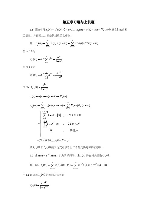
第五章习题与上机题5.1 已知序列12()(),0 1 , ()()()nx n a u n a x n u n u n N =<<=--,分别求它们的自相关函数,并证明二者都是偶对称的实序列。
解:111()()()()()nn mx n n r m x n x n m a u n au n m ∞∞-=-∞=-∞=-=-∑∑当0m ≥时,122()1mmnx n ma r m aaa∞-===-∑ 当0m <时,122()1m mnx n a r m aaa -∞-===-∑ 所以,12()1mx ar m a =-2 ()()()()N x n u n u n N R n =--=22210121()()()()()1,0 =1,00, =()(1)x NN n n N mn N n m N r m x n x n m Rn R n m N m N m N m m Nm N m R m N ∞∞=-∞=-∞--=-=-=-=-⎧=--<<⎪⎪⎪⎪=-≤<⎨⎪⎪⎪⎪⎩-+-∑∑∑∑其他从1()x r m 和2()x r m 的表达式可以看出二者都是偶对称的实序列。
5.2 设()e()nTx n u n -=,T 为采样间隔。
求()x n 的自相关函数()x r m 。
解:解:()()()()e()e ()nTn m T x n n r m x n x n m u n u n m ∞∞---=-∞=-∞=-=-∑∑用5.1题计算1()x r m 的相同方法可得2e()1e m Tx Tr m --=-5.3 已知12()sin(2)sin(2)s s x n A f nT B f nT ππ=+,其中12,,,A B f f 均为常数。
求()x n 的自相关函数()x r m 。
解:解:()x n 可表为)()()(n v n u n x +=的形式,其中)2sin()(11s nT f A n u π=,=)(n v 22sin(2)s A f nT π,)(),(n v n u 的周期分别为 s T f N 111=,sT f N 221=,()x n 的周期N 则是21,N N 的最小公倍数。
数字信号处理教程第四版答案

z2 x (n ) [z ]z 0 8 1 (z )z 4
当n 0时,围线内部没有极点 ,故x(n) 0
1 x(n) 7 u(n 1) 8(n) 4
n
z2 部分分式法: X(z) 1 z 4 X(z) z2 A1 A2 故 1 1 z z (z )z z 4 4
数 字 信 号 处 理
第二章 z变换与离散时间傅里叶 变换(DTFT)
2.2 z变换的定义与收敛域
序列x(ห้องสมุดไป่ตู้)的z变换定义为:
n x ( n ) z
X ( z)
n
对任意给定序列x(n),使其z变换收敛的所有z值的集合 称为X(z)的收敛域,上式收敛的充分必要条件是满足绝 对可和
1 z2 A1 [(z ) ] 1 7 1 4 (z )z z 4 4 z2 A 2 [z ] 8 1 z 0 (z )z 4
n
7 1 X( z ) 8,| z | 1 1 4 1 z 4
1 x(n) 7 u(n 1) 8(n) 4
1 | z | 4
n 1
jIm[z]
1/4 o
Re[z]
当n 1时,分母中z的阶次比分子中 z的阶次高两阶 或两阶以上,可用围线 外部极点求解
1 (z 2)z n 1 1 n x (n ) [(z ) ] 1 7( ) z 1 4 4 4 z 4
z2 当n 0时,F(z) ,此时围线内部有一阶 极点z 0 1 (z )z 4
1 n x (n ) ( ) u (n ) 2
部分分式法: Z[a n u (n )]
1 , | z || a | 1 1 az
数字信号处理课后习题答案(全)1-7章
第 1 章 时域离散信号和时域离散系统
(6) y(n)=x(n2)
令输入为
输出为
x(n-n0)
y′(n)=x((n-n0)2) y(n-n0)=x((n-n0)2)=y′(n) 故系统是非时变系统。 由于
T[ax1(n)+bx2(n)]=ax1(n2)+bx2(n2) =aT[x1(n)]+bT[x2(n)]
第 1 章 时域离散信号和时域离散系统
题4解图(一)
第 1 章 时域离散信号和时域离散系统
题4解图(二)
第 1 章 时域离散信号和时域离散系统
题4解图(三)
第 1 章 时域离散信号和时域离散系统
(4) 很容易证明: x(n)=x1(n)=xe(n)+xo(n)
上面等式说明实序列可以分解成偶对称序列和奇对称序列。 偶对称序列可 以用题中(2)的公式计算, 奇对称序列可以用题中(3)的公式计算。
(2) y(n)=x(n)+x(nN+1)k 0
(3) y(n)= x(k)
(4) y(n)=x(n-nn0)n0
(5) y(n)=ex(n)
k nn0
第 1 章 时域离散信号和时域离散系统
解:(1)只要N≥1, 该系统就是因果系统, 因为输出 只与n时刻的和n时刻以前的输入有关。
如果|x(n)|≤M, 则|y(n)|≤M, (2) 该系统是非因果系统, 因为n时间的输出还和n时间以 后((n+1)时间)的输入有关。如果|x(n)|≤M, 则 |y(n)|≤|x(n)|+|x(n+1)|≤2M,
=2x(n)+x(n-1)+ x(n-2)
将x(n)的表示式代入上式, 得到 1 y(n)=-2δ(n+2)-δ(n+1)-0.5δ(2n)+2δ(n-1)+δ(n-2)
自动化_数字信号处理实验5答案
实验五 IIR滤波器设计一、实验目的1. 掌握冲激响应不变法和双线性变换法设计IIR数字滤波器的原理和方法;2. 观察双线性变换法和冲激响应不变法设计的滤波器的频域特性,了解双线性变换法和冲激响应不变法的特点和区别。
二、实验仪器1. 计算机2. MATLAB软件三、预习要求理解冲激响应不变法,双线性变换法,掌握常用 matlab 程序。
四、实验原理1. IIR数字滤波器一般为线性移不变的因果离散系统,N阶IIR滤波器的传递函数为:,式中系数至少有一个不为0。
IIR数字滤波器的设计通常利用模拟滤波器作为原型滤波器,直接由模拟滤波器的频率响经过冲激响应不变法或双线性变换法转换成IIR数字滤波器。
2. 常用模拟原型滤波器(1)巴特沃斯滤波器巴特沃斯滤波器通带和阻带都单调衰减,所有结束的幅度函数-3dB点为同一点。
其幅度响应为:,式中N为滤波器阶数,通带截止频率。
(2)切比雪夫Ⅰ型滤波器切比雪夫Ⅰ型滤波器在通带呈现等波纹特性,阻带单调衰减,其幅度响应为:,式中N为滤波器阶数;,表示通带波纹大小,越大,波纹越大;为截止频率,不一定为3dB带宽;为N阶Chebyshev多项式。
(3)切比雪夫Ⅱ型滤波器切比雪夫Ⅱ型滤波器在阻带呈现等波纹特性,通带单调衰减,其幅度响应为:,式中是阻带衰减达到一定数值时的最低频率。
(4)椭圆滤波器椭圆滤波器在通带和阻带都呈现波纹特性,在带内均匀波动,具有最快的滚降。
,式中为椭圆函数。
3. 冲激响应不变法所谓冲激响应不变法就是使数字滤波器的单位冲激响应序列等于模拟滤波器的单位冲激响应和的采样值,即:,其中,T为采样周期。
令为模拟系统传递函数,且,则冲激响应不变法得到的数字滤波器传递函数。
冲激响应不变法的特点是:(1)时域逼近特性良好;(2)模拟频率和数字频率呈线性关系。
(3)存在频率混叠效应,故只适用于限带的模拟滤波器。
在 MATLAB 中,可用函数 impinvar 实现从模拟滤波器到数字滤波器的冲激响应不变映射,调用格式为:[bz,az]=impinvar(b,a,fs)[bz,az]=impinvar(b,a)其中,b、a 分别为模拟滤波器的分子和分母多项式系数向量;fs为采样频率(Hz),缺省值 fs=1Hz;bz、az分别为数字滤波器分子和分母多项式系数向量。
数字信号处理课后习题答案(全)1-7章
2. 给定信号:
2n+5
-4≤n≤-1
(x(n)=
6
0
0≤n≤4 其它
(1) 画出x(n)序列的波形, 标上各序列值;
(2) 试用延迟的单位脉冲序列及其加权和表示x(n)序列;
第 1 章 时域离散信号和时域离散系统
(3) 令x1(n)=2x(n-2), 试画出x1(n)波形; (4) 令x2(n)=2x(n+2), 试画出x2(n)波形; (5) 令x3(n)=x(2-n), 试画出x3(n)波形。 解: (1) x(n)序列的波形如题2解图(一)所示。 (2) x(n)=-3δ(n+4)-δ(n+3)+δ(n+2)+3δ(n+1)+6δ(n)
第 1 章 时域离散信号和时域离散系统
题8解图(一)
第 1 章 时域离散信号和时域离散系统
x(n)=-δ(n+2)+δ(n-1)+2δ(n-3)
h(n)=2δ(n)+δ(n-1)+ δ(n-2)
由于
x(n)*δ(n)=x(n)
1
x(n)*Aδ(n-k)=Ax(n-k)
2
故
第 1 章 时域离散信号和时域离散系统
y(n)=x(n)*h(n)
=x(n)*[2δ(n)+δ(n-1)+ δ(n-2) 1 2
, 这是2π有理1数4, 因此是周期序
3
(2) 因为ω=
,
所以
1
8
=16π, 这是无理数, 因此是非周期序列。
2π
第 1 章 时域离散信号和时域离散系统
4. 对题1图给出的x(n)要求:
(1) 画出x(-n)的波形;
数字信号处理实验五答案.doc
1・信号产生函数mstg清单function xt=xtg(N)%实验五信号x(t)产生,并显示信号的幅频特性曲线%xt=xtg产生一个长度为N,冇加性高频噪声的单频调幅信号xt,N二1000., %采样频率Fs二1000Hz%载;波频率fc=Fs/10=100Hz,调制正弦波频率f0=fc/10=10Hz.N=1000;Fs=l000;T=1/Fs;Tp=N*T;t二0:T: (N-1)*T;fc=Fs/10 ;f0=fc/10; %载波频率fc=Fs/10,单频调制信号频率为f0=Fc/10;int=cos (2*pi*f0*t) ; %产生讥频止弦波调制信号mt,频率为f0ct=cos(2*pi*fc*t) ; %产生载波iF弦波信号ct,频率为fc xt=mt. *ct; %相乘产生单频调制信号xtnt=2*rand(l, N)T; %产生随机噪声nI%=======设计高通滤波器hn,用于滤除噪声nt中的低频成分,牛成高通噪声======= fp=150;fs=200;Rp=0. l;As=70; % 滤波器指标fb=[fp, fs] ;m二[0, 1]; % 计算remezord函数所需参数f, m, devdev=[107-As/20), (10" (Rp/20)-l)/(10"(Rp/20)+l)];[n, fo, mo, W]=remezord(fb, m, dev, Fs) ; % 确定rcinezP^i数所盂参数hn=rcmcz (n, fo, mo, W) ; %调用rcme函数进行设计,用J:滤除噪声nt中的低频成分yt二f订ter (hn, 1, 10*nt) ; %滤除随机噪声中低频成分,牛成高通噪声yt%========================以下为绘图部分===================================== xt=xt+yt; %噪声加信号fst=fft(xt, N);k=0:N-l;f=k/Tp;subplot (2, 1, 1) ;plot (t, xt) ;grid;xlabel(' t/s') ;ylabel (' x(t)'); axis([0, Tp/5, min(xt), max(xt)]);titleC (a)信号加噪声波形') subplot (2, 1, 2) ;plot (f, abs(fst)/max(abs (fst))) ;grid; titleC (b)信号加噪声的频谱') axis(f0, Es/2, 0, 1. 2]) ;xlabel C f/Hz');ylabel C if®度') 2•产生FIR数字滤波器设计及软件实现clear all;%==using the function ,xtg£「to plot the picture of xt and its spectrogram==xt=xtg;N=1000;fp=120; fs=150;Rp=0.2;As=60;Fs=1000; %input the defined parameters%to design the filter using th巳Windows methodwc= (fp+fs)/Fs; Ethe cut-off frequence of the filterB=2*pi*(fs-fp)/Fs; %the width of prototype filterNb=cei丄(11*pi/B); %the length of window of blackmanhn=f ir1 (Nb-1,wc,blackman(Nb));Hw=abs(fft(hn,1024)); % the frequency characteristic of the filter ywt = f ft f i]_t (hn z xt』N);%to filter xt using fftfilt%to draw the figure using the Windows methodf=[0:1023]*Fs/1024; ~figure (2)subplot(2f1,1);plot(f,20*logl0(Hw/max (Hw)));grid;xlabel ( 1f/Hz 1);ylabel(1 Amplitude 1);title ( 1 the frequency characteristic of the low-pass filter 1); axis ( [0,Fs/2z-120, 20]);t=[0:N-1]/Fs;Tp=N/Fs;subplot (2f1,2);plot (t,ywt);grid;xlabel(1t/s1);ylabel(1y_w(t) T);title ( 1 the signal waves after filtering noises 1);axis([0,Tp/2,-1,1]);%to design the filter using the best uniform approximation method fb=[fp z fs];m=[1,0];% define the parameters of remezorddev=[ (10A (Rp/20)-1)/(10A(Rp/20)+1),10A(-As/20)];[Ne z fo, mo z W]=remezord(fb,m, dev,Fs); %define the parameters of remez hn=remez(Ne,fmo z W);Hw=abs(fft(hn z1024)); % the frequency characteristic of the filteryet=fft£i1t(hn/Xt’N);%to filter xt using filt%to draw the figure using the best uniform approximation methodf igure(3);subplot(2,1,1);f=[0:1023]*Fs/1024;plot (f, 20*logl0 (Hw/max (Hw) ) ) ; grid; xlabel ( 1 f/Hz ' ) ; ylabel ( f Amplitude 1 ); title ( 1 the frequency characteristic of the low-pass filter 1);axis([0,Fs/2,-80,10]);subplot (2, 1 z 2 ) ; plot (t, yet) ; grid; xlabel ( 11/s ' ) ; ylabel ( ' y_e (t) 1 ); title ( 1 the signal waves after filtering noises');axis([0,Tp/2,-1,1]);⑻信号加噪声波形105e oX-5-100 0.02 0.04 0.06 0.08 0.1 0.12 0.14 0.16 0.18 0.2t/s(b)信号加噪声的频谱1® 0.50 50 100 150 200 250 300 350 400 450 500f/Hz-800 50 100 150 200 250 300 350400 450 500f/Hzthe signal waws after filtering noises050.5 0 0 0.05 0.1 0.15 0.2 0.250.3 0.35 0.4 0.45 0.5 t/s 0-20-40-60the frequency characteristic of the low-pass filter。
数字信号处理习题及解答..
X (e j0 )
n 3
x ( n) 6
x(n)e jn
7
π
π
X (e j )d x(0) 2π 4π
X (e jπ )
n
n 3
7
(1) n x(n) 2
数字信号处理习题及解答
第三章 信号的傅里叶变换 2 试求如下序列的傅里叶变换: (1) x1(n)=δ(n-3)
第一章离散时间信号与离散时间系统数字信号处理习题及解答2解答第一章离散时间信号与离散时间系统数字信号处理习题及解答3第一章离散时间信号与离散时间系统数字信号处理习题及解答3解答第一章离散时间信号与离散时间系统数字信号处理习题及解答4第一章离散时间信号与离散时间系统数字信号处理习题及解答4解答第一章离散时间信号与离散时间系统数字信号处理习题及解答4解答第一章离散时间信号与离散时间系统数字信号处理习题及解答1第二章z变换及离散时间系统分析数字信号处理习题及解答1解答第二章z变换及离散时间系统分析数字信号处理习题及解答1解答第二章z变换及离散时间系统分析数字信号处理习题及解答2第二章z变换及离散时间系统分析数字信号处理习题及解答2解答第二章z变换及离散时间系统分析数字信号处理习题及解答2解答第二章z变换及离散时间系统分析数字信号处理习题及解答2第二章z变换及离散时间系统分析数字信号处理习题及解答2解答第二章z变换及离散时间系统分析数字信号处理习题及解答2解答第二章z变换及离散时间系统分析数字信号处理习题及解答2解答第二章z变换及离散时间系统分析数字信号处理习题及解答2解答第二章z变换及离散时间系统分析数字信号处理习题及解答3已知第二章z变换及离散时间系统分析112122113??????zzzx求出对应xz的各种可能的序列表达式
数字信号处理作业 第五章 参考答案

(1) 由极点构成 H a ( s ) 的分母多项式,分子为分母多项式的常数。 (2) H a ( s ) 展成部分分式。 (3) 据有理分式变换得到对应的 H ( z ) 各分式,整理得到最后的 H ( z ) 。 22、 取 T=1, 预畸, 由已知列出对模拟滤波器的衰减要求, 解出 N=6.04, 取 N=7, 得到
−0.5
Z −1
−1
0.9
−0.81
4、 H ( z ) = −4.9383 +
2.1572 4.7811 − 1.5959 z −1 + 1 + 0.5 z −1 1 − 0.9 z −1 + 0.81z −2
−4.9383
x ( n) y ( n)
2.1572 −0.5
Z −1
4.7811
Z
0.9 −0.81
= H 2 ( z)
α 02 + α12 z -1 -3.1986 + 0.2591z -1 = 1 +z 2 1 + 1.618 z - 4π 2 2 1 + r z 1 - 2rz -cos 5
频率取样型实现流程图:
−10.125
Z −1
18.3236
x ( n)
Z −1
x ( n)
Z −1
Z −1
+
Z −1
− 7 4
+
Z −1
− 69 8
+
y ( n) 4) 频率取样型:取 r=1,N=5,得到 DFT{h(n)}为:
{-10.1250 9.1618 + 6.6564i -1.5993 - 4.9221i -1.5993 + 4.9221i 9.1618 - 6.6564i}
数字信号处理习题答案及matlab实验详解.pdf
Z = 0,0.8361,0.4306 P =1.0000, 0.6000,0.3000
(2)
由于 H (z)
Y (z) X (z)
1
3 1.9
3.8z1 1.08 z1 1.08z2
z 2 0.18z
3
所以系统的差分方程:
y(n) 1.9 y(n 1) 1.08 y(n 2) 0.18 y(n 3) 3x(n) 3.8x(n 1) 1.08x(n 2)
1 2
n
u(n),
x
2
(n)
1 3
n
u
(n)
利用 Z 变换性质求 y(n)的 Z 变换 Y(Z)。
实验 2-1 离散系统的分析的基本理论 实验目的:加深对离散系统基本理论和方法的理解
1 一线性移不变离散时间系统的单位抽样响应为 h(n) (1 0.3n 0.6n )u(n)
(1) 求该系统的转移函数 H (z) ,并画出其零-极点图; (2) 写出该系统的差分方程。
阶跃响应为: y[n] x[n] h[n] x[m]h[n m] h(n m), n m, m 0
m
m0
即 y(0) 0, y(1) 0.25, y(2) 0.5, y(3) 0.75,其余y(n) 1, (n 3)
利用函数 h=impz(b,a,N)和 y=filter(b,a,x)分别绘出冲激和阶跃响应 b=[0,0.25,0.25,0.25,0.25]; a=1; x=ones(1,100); h=impz(b,a,100);y=filter(b,a,x) figure(1) subplot(2,1,1); stem(h,’.’); subplot(2,1,2); plot(y,’.’);
数字信号处理课后习题答案(全)1-7章
最后结果为 0
n<0或n>7
y(n)= n+1 0≤n≤3 8-n 4≤n≤7
y(n)的波形如题8解图(一)所示。 (2) y(n) =2R4(n)*[δ(n)-δ(n-2)]=2R4(n)-2R4(n-2)
=2[δ(n)+δ(n-1)-δ(n+4)-δ(n+5) y(n)的波形如题8解图(二)所示
因此系统是非线性系统。
第 1 章 时域离散信号和时域离散系统
(6) y(n)=x(n2)
令输入为
输出为
x(n-n0)
y′(n)=x((n-n0)2) y(n-n0)=x((n-n0)2)=y′(n) 故系统是非时变系统。 由于
T[ax1(n)+bx2(n)]=ax1(n2)+bx2(n2) =aT[x1(n)]+bT[x2(n)]
因此系统是非时变系统。
第 1 章 时域离散信号和时域离散系统
(5) y(n)=x2(n)
令输入为
输出为
x(n-n0)
y′(n)=x2(n-n0) y(n-n0)=x2(n-n0)=y′(n) 故系统是非时变系统。 由于
T[ax1(n)+bx2(n)]=[ax1(n)+bx2(n)]2 ≠aT[x1(n)]+bT[x2(n) =ax21(n)+bx22(n)
第 1 章 时域离散信号和时域离散系统
题4解图(一)
第 1 章 时域离散信号和时域离散系统
题4解图(二)
第 1 章 时域离散信号和时域离散系统
题4解图(三)
第 1 章 时域离散信号和时域离散系统
(4) 很容易证明: x(n)=x1(n)=xe(n)+xo(n)
(2021年整理)数字信号处理习题集(附答案)
数字信号处理习题集(附答案)(推荐完整)编辑整理:尊敬的读者朋友们:这里是精品文档编辑中心,本文档内容是由我和我的同事精心编辑整理后发布的,发布之前我们对文中内容进行仔细校对,但是难免会有疏漏的地方,但是任然希望(数字信号处理习题集(附答案)(推荐完整))的内容能够给您的工作和学习带来便利。
同时也真诚的希望收到您的建议和反馈,这将是我们进步的源泉,前进的动力。
本文可编辑可修改,如果觉得对您有帮助请收藏以便随时查阅,最后祝您生活愉快业绩进步,以下为数字信号处理习题集(附答案)(推荐完整)的全部内容。
数字信号处理习题集(附答案)(推荐完整)编辑整理:张嬗雒老师尊敬的读者朋友们:这里是精品文档编辑中心,本文档内容是由我和我的同事精心编辑整理后发布到文库,发布之前我们对文中内容进行仔细校对,但是难免会有疏漏的地方,但是我们任然希望数字信号处理习题集(附答案)(推荐完整) 这篇文档能够给您的工作和学习带来便利。
同时我们也真诚的希望收到您的建议和反馈到下面的留言区,这将是我们进步的源泉,前进的动力。
本文可编辑可修改,如果觉得对您有帮助请下载收藏以便随时查阅,最后祝您生活愉快业绩进步,以下为〈数字信号处理习题集(附答案)(推荐完整)〉这篇文档的全部内容。
第一章数字信号处理概述简答题:1.在A/D变换之前和D/A变换之后都要让信号通过一个低通滤波器,它们分别起什么作用?答:在A/D变化之前让信号通过一个低通滤波器,是为了限制信号的最高频率,使其满足当采样频率一定时,采样频率应大于等于信号最高频率2倍的条件。
此滤波器亦称位“抗折叠”滤波器。
在D/A变换之后都要让信号通过一个低通滤波器,是为了滤除高频延拓谱,以便把抽样保持的阶梯形输出波平滑化,故友称之为“平滑”滤波器。
判断说明题:2.模拟信号也可以与数字信号一样在计算机上进行数字信号处理,自己要增加一道采样的工序就可以了. ( )答:错。
需要增加采样和量化两道工序。
数字信号处理第四版高西全课后答案

(1)y(n)=x(n)+2x(n-1)+3x(n-2) (2)y(n)=2x(n)+3 (3)y(n)=x(n-n0) n0 (4)y(n)=x(-n)
第 1 章 时域离散信号和时域离散系统
故延时器是线性系统。
第 1 章 时域离散信号和时域离散系统
(4) y(n)=x(-n)
令输入为
输出为
x(n-n0)
y′(n)=x(-n+n0) y(n-n0)=x(-n+n0)=y′(n) 因此系统是线性系统。 由于
T[ax1(n)+bx2(n)]=ax1(-n)+bx2(-n) =aT[x1(n)]+bT[x2(n)]
第 1 章 时域离散信号和时域离散系统
题4解图(一)
第 1 章 时域离散信号和时域离散系统
题4解图(二)
第 1 章 时域离散信号和时域离散系统
题4解图(三)
第 1 章 时域离散信号和时域离散系统
(4) 很容易证明: x(n)=x1(n)=xe(n)+xo(n)
上面等式说明实序列可以分解成偶对称序列和奇对称序列。 偶对称序列可 以用题中(2)的公式计算, 奇对称序列可以用题中(3)的公式计算。
所以 T[ax1(n)+bx2(n)]=aT[x1(n)]+bT[x2(n)]
第 1 章 时域离散信号和时域离散系统
(2) 令输入为
输出为
x(n-n0)
y′(n)=2x(n-n0)+3 y(n-n0)=2x(n-n0)+3=y′(n) 故该系统是非时变的。 由于
《数字信号处理(第四版)》部分课后习题解答
《数字信号处理(第四版)》部分课后习题解答一、简答题1. 什么是数字信号处理?数字信号处理(DSP)是指对数字信号进行处理和分析的一种技术。
它使用数学和算法处理模拟信号,从而实现信号的采样、量化、编码、存储和重构等过程。
DSP广泛应用于通信、音频处理、图像处理和控制系统中。
2. 数字信号处理的主要特点有哪些?•数字信号处理能够处理和分析具有广泛频谱范围的信号。
•数字信号处理能够实现高精度的信号处理和复杂的算法运算。
•数字信号处理能够实现信号的存储、传输和复原等功能。
•数字信号处理可以利用计算机等处理硬件进行实时处理和系统集成。
3. 数字信号处理的基本原理是什么?数字信号处理的基本原理是将连续时间的模拟信号转换成离散时间的数字信号,然后通过一系列的算法对数字信号进行处理和分析。
该过程主要涉及信号的采样、量化和编码等环节。
4. 什么是离散时间信号?离散时间信号是指信号的取样点在时间上呈现离散的情况。
在离散时间信号中,只能在离散时间点上获取信号的取样值,而无法观测到连续时间上的信号变化。
5. 描述离散时间信号的功率和能量的计算方法。
对于离散时间信号,其功率和能量的计算方法如下:•功率:对于离散时间信号x(n),其功率可以通过求平方和的平均值来计算,即功率P = lim(T->∞) [1/T *∑|x(n)|^2],其中T表示信号x(n)的观测时间。
•能量:对于离散时间信号x(n),其能量可以通过求平方和来计算,即能量E = ∑|x(n)|^2。
二、计算题1. 设有一个离散时间周期序列x(n) = [2, 3, -1, 4, 0, -2],求其周期N。
由于x(n)是一个周期序列,我们可以通过观察序列来确定其周期。
根据观察x(n)的取值,我们可以发现序列在n=1和n=5两个位置上取得了相同的数值。
因此,序列x(n)的周期为N = 5 - 1 = 4。
2. 设有一个信号x(t) = 2sin(3t + π/4),请将其离散化为离散时间信号x(n)。
数字信号处理 Chapter05答案

2011/4/10
3
Notice: Skipped Sections
5.7 5.8 (all) 5.9 (all) 5.10 5.11
2011/4/10
4
5.1
Introduction
2011/4/10
5
5.1 Introduction
Digital processing of a real-world continuous-time signal involves the following basic steps:
The multiplication operation yields an impulse train
Note: Analog Filters are very important for digital systems. Since both the anti-aliasing filter and the reconstruction filter are analog lowpass filters, we review first the theory behind the design of such filters Also, the most widely used IIR digital filter design method is based on the conversion of an analog lowpass prototype
g[n ] = ga (nT ), -¥ <n < ¥
(5.1)
With T being the sampling period. The reciprocal of T is called the sampling frequency , i.e., 1⁄ . It is known that the frequency-domain of the analog signal is given by its FT:
《数字信号处理》课后答案

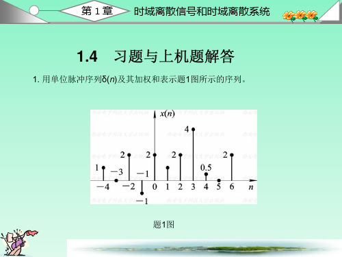
数字信号处理课后答案 1.2 教材第一章习题解答1. 用单位脉冲序列()n δ及其加权和表示题1图所示的序列。
解:()(4)2(2)(1)2()(1)2(2)4(3)0.5(4)2(6)x n n n n n n n n n n δδδδδδδδδ=+++-+++-+-+-+-+-2. 给定信号:25,41()6,040,n n x n n +-≤≤-⎧⎪=≤≤⎨⎪⎩其它(1)画出()x n 序列的波形,标上各序列的值; (2)试用延迟单位脉冲序列及其加权和表示()x n 序列; (3)令1()2(2)x n x n =-,试画出1()x n 波形; (4)令2()2(2)x n x n =+,试画出2()x n 波形; (5)令3()2(2)x n x n =-,试画出3()x n 波形。
解:(1)x(n)的波形如题2解图(一)所示。
(2)()3(4)(3)(2)3(1)6()6(1)6(2)6(3)6(4)x n n n n n n n n n n δδδδδδδδδ=-+-+++++++-+-+-+-(3)1()x n 的波形是x(n)的波形右移2位,在乘以2,画出图形如题2解图(二)所示。
(4)2()x n 的波形是x(n)的波形左移2位,在乘以2,画出图形如题2解图(三)所示。
(5)画3()x n 时,先画x(-n)的波形,然后再右移2位,3()x n 波形如题2解图(四)所示。
3. 判断下面的序列是否是周期的,若是周期的,确定其周期。
(1)3()cos()78x n A n ππ=-,A 是常数;(2)1()8()j n x n e π-=。
解:(1)3214,73w w ππ==,这是有理数,因此是周期序列,周期是T=14; (2)12,168w wππ==,这是无理数,因此是非周期序列。
5. 设系统分别用下面的差分方程描述,()x n 与()y n 分别表示系统输入和输出,判断系统是否是线性非时变的。
数字信号处理米特拉第四版实验四答案
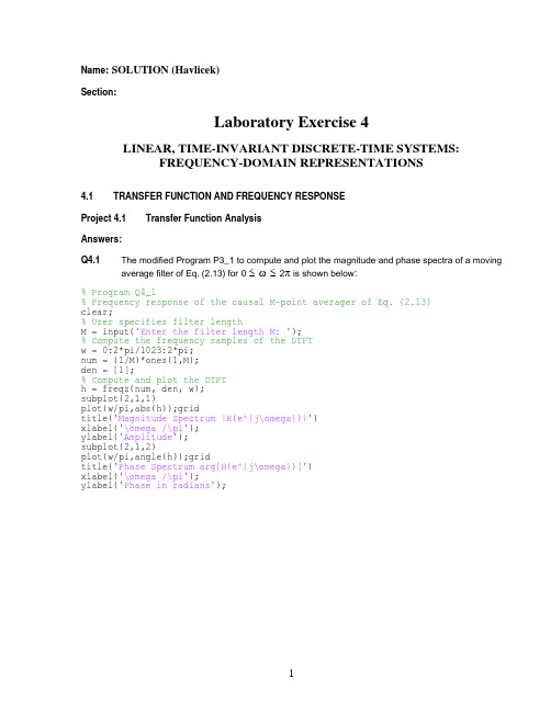
Q4.5
The plots of the first 100 samples of the impulse responses of the two filters of Questions 4.2
3
2
1
0
-1 0 0.1 0.2 0.3 0.4 0.5 0.6 0.7 0.8 0.9 1 /
From this plot we make the following observations: Usually, it is desirable for a filer to have an approximately linear phase in the passband, which is the same thing as an approximately constant group delay in the passband. This filter is notch filter; it is a bandstop filter with a narrow stopband centered at a normalized frequency just below 0.3. From the graph above, we see that the group delay is approximately constant over much of the passband.
M=3
Magnitude Spectrum |H(ej)| 1
0.5
0 0 0.2 0.4 0.6 0.8 1 1.2 1.4 1.6 1.8 2 / Phase Spectrum arg[H(ej)]
4 2 0 -2 -4
0 0.2 0.4 0.6 0.8 1 1.2 1.4 1.6 1.8 2 /
数字信号处理实验指导书思考题答案实验图

目录实验一 Matlab与数字信号处理基础 (2)实验二离散傅里叶变换与快速傅里叶变换 (4)实验三数字滤波器结构 (6)注释 (9)主要参考文献 (9)实验一 Matlab与数字信号处理基础一、实验目的和任务1、熟悉Matlab的操作环境2、学习用Matlab建立基本序列的方法;3、学习用仿真界面进行信号抽样的方法。
二、实验内容1、基本序列的产生:单位抽样序列、单位阶跃序列、矩形序列、实指数序列和复指数序列的产生2、用仿真界面进行信号抽样练习:用simulink建模仿真信号的抽样三、实验仪器、设备及材料计算机、Matlab软件四、实验原理序列的运算、抽样定理五、主要技术重点、难点Matlab的各种命令与函数、建模仿真抽样定理六、实验步骤1、基本序列的产生:单位抽样序列δ(n): n=-2:2;x=[0 0 1 0 0];stem(n,x);单位阶跃序列u(n):n=-10:10;x=[zeros(1,10) ones(1,11)];stem(n,x);矩形序列R N(n):n=-2:10;x=[0 0 ones(1,5) zeros(1,6)];stem(n,x);实指数序列0.5n:n=0:30;x=0.5.^nstem(n,x);复指数序列e(-0.2+j0. 3)n:n=0:30;x=exp((-0.2+j*0.3)*n);模:stem(n,abs(x));幅角:stem(n,angle(x));2、用仿真界面进行信号抽样练习:(1)在Matlab命令窗口中输入simulink 并回车,以打开仿真模块库;(2)按CTRL+N,以新建一仿真窗口;在仿真模块库中用鼠标点击Sources(输入源模块库),从中选择sine wave(正弦波模块)并将其拖至仿真窗口;(3)在仿真模块库中用鼠标点击Discrete(离散模块库),从中选择Zero-Order Hold(零阶保持器模块)并将其拖至仿真窗口;(4)在仿真模块库中用鼠标点击Sinks(显示模块库),从中选择Scope(示波器模块)并将其拖至仿真窗口;(5)在仿真窗口中把上述模块依次连接起来;(6)用鼠标双击Scope模块,以打开示波器的显示界面;(7)用鼠标点击仿真窗口工具条中的►图标开始仿真,结果显示在示波器中;(8)用鼠标双击Zero-Order Hold模块,打开其参数设置窗口,改变sample time参数值,例如1、0.5、0.1、0.05…,用鼠标点击仿真窗口工具条中的►图标开始仿真,比较示波器显示结果(选三个参数值,得三个结果);(9)在仿真模块库中用鼠标点击Sinks(显示模块库),从中选择To Workspace(输出到当前工作空间的变量模块)并将其拖至仿真窗口;(10)用鼠标双击To Workspace模块,打开其参数设置窗口,改变variable name参数值为x ;同时把save format参数值设置为Array ;(11)在仿真窗口中先用鼠标点击Zero-Order Hold模块与Scope模块的连线,然后按住CTRL 键,从选中连线的中部引出一条线到To Workspace模块;(12)用鼠标双击Zero-Order Hold模块,打开其参数设置窗口,改变sample time参数值,例如1、0.5、0.1、0.05…,用鼠标点击仿真窗口工具条中的►图标开始仿真,并返回命令窗口,用stem(x)作图,比较序列图显示结果(选三个参数值,得三个结果);七、实验报告要求1、实验步骤按实验内容指导进行;2、对于实验内容1和2的数据必须给出的离散图,其相关参数应在图中注明;3、具有关联性和比较性的图形最好用subplot()函数,把它们画在一起;4、实验报告按规定格式填写,要求如下:(1)实验步骤根据自己实际操作填写;(2)各小组实验数据不能完全相同,否则以缺席论处;5、实验结束,实验数据交指导教师检查,得到允许后可以离开,否则以缺席论处;八、实验注意事项1、Matlab编程、文件名、存盘目录均不能使用中文。
数字信号处理课后习题答案 全全全
1
1 >
. . z
z
(3) , | | 0.5
1 0.5
1
1 <
. . z
z
(4)
, | | 0
1 0.5
1 (0.5 )
1
1 10
>
.
.
.
.
z
z
z
1.8 (1) ) , 0
1
( ) (1 2
1 3 3
3.014 2.91 1.755 0.3195
0.3318 0.9954 0.9954 0.3318
1 0.9658 0.5827 0.1060
z z z
z z z
z z z
z z z
. . .
. . .
. . .
. . .
. + .
=
= . . +
= . . . +
..
.
..
. π
2.13
0,1,2, , 1
( ) ( )
= .
=
k N
Y rk X k
..
2.14
Y(k) = X ((k)) R (k) k = 0,1, ,rN .1 N rN ..
2.15 (1) x(n) a R (n) N
= n y(n) b R (n) N
= n
(2) x(n) =δ (n) y(n) = Nδ (n)
2.16 ( )
1
1 a R N
a N
n
. N
- 1、下载文档前请自行甄别文档内容的完整性,平台不提供额外的编辑、内容补充、找答案等附加服务。
- 2、"仅部分预览"的文档,不可在线预览部分如存在完整性等问题,可反馈申请退款(可完整预览的文档不适用该条件!)。
- 3、如文档侵犯您的权益,请联系客服反馈,我们会尽快为您处理(人工客服工作时间:9:00-18:30)。
50
100
150
200
250
Time index n
T = 0.02 msec
Continuous-time signal xa(t) 1
0.5
0
-0.5
-1 0 0.1 0.2 0.3 0.4 0.5 0.6 0.7 0.8 0.9 1 Time, msec Discrete-time signal x[n]
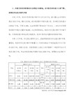
Q5.5 The plots of the continuous-time sinusoidal signal of frequency 3 kHz and its sampled version
generated by running a modified Program P5_1 are shown below: (NOTE: the book is in error about the frequency. Since the “t” in the program is in units of msec, the frequency here is 3 kHz, not 3 Hz.)
Time index n
Amplitude
Based on these results we make the following observations – In all three cases, we have T = 0.1 msec. Originally, in Q5.1. we had f = 13kHz. This gives a maximum sampling period of 1/26 » 0.0385 msec to satisfy the Nyquist criterion, as we observed above.
0 0.5 1 1.5 2 2.5 3 3.5 4 4.5 5 Time index n
Amplitude
Amplitude
4
Based on these results we make the following observations – Since the “analog” waveform goes through 13 cycles in the 1 msec shown in the graph, there will be aliasing unless we get at least two samples per cycle, or 26 samples total on the graph. 26 samples in 1 msec is a sampling rate of 26 kHz, which requires T < 1/26 » 0.0385 msec to avoid
aliasing. With T=0.004 msec. there is no aliasing and the discrete-time waveform has an appearance that is very similar to that of the “analog” waveform. With T=0.02 msec, there is still no aliasing, but the sampling rate is much closer to being “critical,” i.e., much closer to the Nyquist rate. Consequently, the appearance of the discrete-time waveform is less similar to the “analog waveform,” although perfect reconstruction is still possible. With T=0.15 msec, there is significant aliasing and the discrete-time waveform has the appearance of an “analog” waveform of much lower frequency. Finally, with T=0.2 msec, there is again severe aliasing which causes the discrete-time waveform to have the appearance of an “analog” waveform of lower frequency.
The sampling period in seconds is - T = 0.1 msec.
Q5.3 The effects of the two axis commands are – The first axis command sets the minimum and maximum values for the x-axis and the y-axis in the upper plot. The second axis command does the same thing for the lower plot. In each axis command, the first two parameters are the minimum and maximum values for the x-axis. The third and fourth parameters are the minimum and maximum values for the y-axis.
Q5.4
The plots of the continuous-time signal and its sampled version generated by running Program
P5_1 for the following four values of the sampling period are shown below:
Amplitude
Continuous-time signal xa(t) 1
0.5
0
-0.5
-1 0 0.1 0.2 0.3 0.4 0.5 0.6 0.7 0.8 0.9 1 Time, msec Discrete-time signal x[n]
1
0.5
0
-0.5
-1
0
1
2
3
4
5
6
7
8
9 10
2
Amplitude
Amplitude
T = 0.004 msec
1 0.5
0 -0.5
-1 0
1 0.5
0 -0.5
-1 0
Continuous-time signal xa(t)
0.1 0.2 0.3 0.4 0.5 0.6 0.7 0.8 0.9 1 Time, msec
Discrete-time signal x[n]
1
Answers:
Q5.1
The plots of the continuous-time signal and its sampled version generated by running Program
P5_1 are shown below:
Amplitude
Continuous-time signal xa(t) 1
A copy of Program P5_1 is given below:
% Program P5_1 % Illustration of the Sampling Process % in the Time-Domain clf; t = 0:0.0005:1; f = 13; xa = cos(2*pi*f*t); subplot(2,1,1) plot(t,xa);grid xlabel('Time, msec');ylabel('Amplitude'); title('Continuous-time signal x_{a}(t)'); axis([0 1 -1.2 1.2]) subplot(2,1,2); T = 0.1; n = 0:T:1; xs = cos(2*pi*f*n); k = 0:length(n)-1; stem(k,xs);grid; xlabel('Time index n');ylabel('Amplitude'); title('Discrete-time signal x[n]'); axis([0 (length(n)-1) -1.2 1.2])
1
0.5
0
-0.5
-1
0
1
2
3
4
5
6
Time index n
T = 0.2 msec
Continuous-time signal xa(t) 1 0.5 0 -0.5 -1
0 0.1 0.2 0.3 0.4 0.5 0.6 0.7 0.8 0.9 1 Time, msec
Discrete-time signal x[n] 1 0.5 0 -0.5 -1
Time index n
Amplitude
5
The plots of the continuous-time sinusoidal signal of frequency 7 kHz and its sampled version
generated by running a modified Program P5_1 are shown below: (Again, the book is in error. For the same reason as above, the frequency here is 7 kHz, not 7 Hz.)