基于排队理论的仿真模型
运筹学实验8、用EXCEL进行排队问题仿真

实验八、基于Excel的排队问题仿真排队问题常常连续地或并行地发生(例如在装配线和工作车间),通常无法用建立数学模型的方法解决。
然而,排队问题通常容易在计算机上进行仿真。
下面我们通过一个两阶段装配线的例子阐述如何借助于Excel建立一个排队问题的仿真模型。
一、实验目的1、掌握如何用Excel建立排队问题仿真模型;2、读懂Excel输出的运算结果,并用于指导实践。
二、实验内容两阶段装配线问题一条装配线所组装的产品体积可能很大,例如:冰箱、空调机、汽车、电视机或家具、图1表示的是一条装配线上的两个工作站。
产品的体积是装配线分析和设计所要考虑的一个重要因素,因为每个工作站上所能存放的产品数量将会影响工人的工作。
如果产品体积很大,那么相邻的工作站存在着相互依赖的关系。
如图1所示,鲍博和雷在一个两阶段装配线上工作,鲍博在工作站1上装配完的产品传递给工作站2上的雷,雷再进行加工。
如果两个工作站相连,中间没有存入半成品的地方,那么鲍博如果干得慢,雷就会被迫等待;相反,如果鲍博和干得快(或者说雷完成工作比鲍博用时长),那么鲍博就得等雷。
在这个仿真问题中,我们假设鲍博是组装线上的第一个工人,他能够在任何时候拿到需组装的半成品进行工作。
那么,我们把分析重点放在鲍博与雷彼此之间的相互影响上。
1、研究的目标:关于这条装配线,我们希望能通过研究解决一些问题。
下面是我们列出的部分待解决的问题:○每个工人的平均完工时间是多少?○这条组装线的生产率是多少?○鲍博等待雷的时间是多少?○雷等待鲍博的时间是多少?○如果两个工作站中间的空间加大,可以存储半成品,从而增加了工人的独立性,那么这对于生产率、等待时间等问题会有什么影响?2、数据的采集:进行系统仿真,我们需要鲍博和雷的装配时间数据。
要收集这些数据,一种方法就是将总装配时间分割成小段时间,在每段时间对工人进行单独观测。
对这些数据进行简单的汇总和分析,我们可以得到非常有用的直方图。
基于MatLab的排队系统仿真研究

/(-  ̄ 1p) 一
客户到达
— — — — — — —
— — — 型 H 器 童 f l I — — — 丽辑 —圭 —塑— 1 — —4 — — ~
f ) / c 统 的 数 学 特 性 3 M M, 系 M M/ 的 排 队 系 统 有 c台服 务 器 . 台服 务 器 独 立 / e 每 工 作 . 具 有 相 同分 布 的 服 务 时 间 , 们 假 设 所 有 服 务 且 我
0 引 言
排 队论 是 研 究 系 统 由于 随 机 因 素 的干 扰 而 出 现 排 队现 象 的一 门学 科 排 队是 日常 生 活 中经 常 遇 到 的 现 象 。例 如 : 出行 坐 火 车等 待 检票 进 站 的 排 队 ; 食 堂 打 到 饭所 形成的排 队 ; 校 打预防针 , 检所 形成 的排 队 ; 学 体 看 电影 、 游 时前 往售 票 处 购 票 形 成 的排 队等 。 近 几 旅 最
服 务 效 率 与 最合 理 的 配 置 。应 用 Ma a t b对 M/ c M / / / 等排 队 系 统进 行 仿 真 , 仿 L M/ , M c N 对
真 结 果进 行 评 估 , 果 表 明 , 方 法是 切 实 可行 的。 结 该
关 键 词 :仿 真 ;MaL b¥言 ;排 队 系统 ;马可 夫过 程 ta i
图 1 单 服 务 台 排 队 系 统 的 结构 模 型
台是空 的概率 P, n所有服务 台都在忙 的概率 P , 由下面
12 排 队 系统 的数 学特 性 .
( ) 人记 号 和重 要 度 量 参 数 1引
收 稿 日期 :0 0 7 2 2 1 —0 ~ 0 修 稿 日期 :0 0 0 —1 21— 8 1
MM1排队系统仿真matlab试验报告
M/M/1排队系统实验报告一、实验目的本次实验要求实现M/M/1单窗口无限排队系统的系统仿真,利用事件调度法实现离散事件系统仿真,并统计平均队列长度以及平均等待时间等值,以与理论分析结果进行对比。
二、实验原理根据排队论的知识我们知道,排队系统的分类是根据该系统中的顾客到达模式、服务模式、服务员数量以及服务规则等因素决定的。
1、顾客到达模式设到达过程是一个参数为入的Poisson过程,则长度为t的时间内到达k个呼p (t)=(入“ e 4叫的概率服从Poisson分布,即k k!,k = 01,2, .. ,其中入>0为一常数,表示了平均到达率或Poisson呼叫流的强度。
2、服务模式设每个呼叫的持续时间为二,服从参数为N的负指数分布,即其分布函数为P{ X < t } = 1 - e-k t > 03、服务规则先进先服务的规则(FIFO)4、理论分析结果入P = Q = -2—在该M/M/1系统中,设口,则稳态时的平均等待队长为Q 1-P,顾客上乙T T T T =的平均等待时间为N-九。
三、实验内容M/M/1排队系统:实现了当顾客到达分布服从负指数分布,系统服务时间也服从负指数分布,单服务台系统,单队排队,按FIFO (先入先出队列)方式服务。
四、采用的语言MatLab语言源代码:clear;clc;%M/M/1排队系统仿真SimTotal=input('请输入仿真顾客总数SimTotal='); %仿真顾客总数;Lambda=0.4; % 到达率 Lambda;Mu=0.9; % 服务率 Mu;t_Arrive=zeros(1,SimTotal);t_Leave=zeros(1,SimTotal);ArriveNum=zeros(1,SimTotal);LeaveNum=zeros(1,SimTotal);Interval_Arrive=-log(rand(1,SimTotal))/Lambda;% 到达时间间隔Interval_Serve=-log(rand(1,SimTotal))/Mu;% 服务时间 t_Arrive(1)=Interval_Arrive(1);% 顾客到达时间ArriveNum(1)=1;for i=2:SimTotalt_Arrive(i)=t_Arrive(i-1)+Interval_Arrive(i);ArriveNum(i)=i;endt_Leave(1)=t_Arrive(1)+Interval_Serve(1);% 顾客离开时间 LeaveNum(1)=1;for i=2:SimTotalif t_Leave(i-1)<t_Arrive(i)t_Leave(i)=t_Arrive(i)+Interval_Serve(i);elset_Leave(i)=t_Leave(i-1)+Interval_Serve(i);endLeaveNum(i)=i;endt_Wait=t_Leave-t_Arrive; %各顾客在系统中的等待时间 t_Wait_avg=mean(t_Wait);t_Queue=t_Wait-Interval_Serve;%各顾客在系统中的排队时间 t_Queue_avg=mean(t_Queue);Timepoint=[t_Arrive,t_Leave];%系统中顾客数随时间的变化Timepoint=sort(Timepoint);ArriveFlag=zeros(size(Timepoint));% 至 U达时间标志CusNum=zeros(size(Timepoint));temp=2;CusNum(1)=1;for i=2:length(Timepoint)if (temp<=length(t_Arrive))&&(Timepoint(i)==t_Arrive(temp)) CusNum(i)=CusNum(i-1)+1;temp=temp+1;ArriveFlag(i)=1;elseCusNum(i)=CusNum(i-1)-1;endend%系统中平均顾客数计算Time_interval=zeros(size(Timepoint));Time_interval(1)=t_Arrive(1);for i=2:length(Timepoint)Time_interval(i)=Timepoint(i)-Timepoint(i-1);endCusNum_fromStart=[0 CusNum];CusNum_avg=sum(CusNum_fromStart.*[Time_interval 0] )/Timepoint(end);QueLength=zeros(size(CusNum));for i=1:length(CusNum)if CusNum(i)>=2QueLength(i)=CusNum(i)-1;elseQueLength(i)=0;endendQueLength_avg=sum([0 QueLength].*[Time_interval 0] )/Timepoint(end);% 系统平均等待队长%仿真图figure(1);set(1,'position',[0,0,1000,700]);subplot(2,2,1);title('各顾客到达时间和离去时间’);stairs([0 ArriveNum],[0 t_Arrive],'b');hold on;stairs([0 LeaveNum],[0 t_Leave],'y');legend('到达时间‘,‘离去时间’); hold off;subplot(2,2,2);stairs(Timepoint,CusNum,'b')title('系统等待队长分布');xlabel('时间');ylabel('队长’); subplot(2,2,3);title('各顾客在系统中的排队时间和等待时间’);stairs([0 ArriveNum],[0 t_Queue],'b');hold on;stairs([0 LeaveNum],[0 t_Wait],'y');hold off;legend('排队时间‘,‘等待时间’);%仿真值与理论值比较disp(['理论平均等待时间t_Wait_avg=',num2str(1/(Mu-Lambda))]);disp(['理论平均排队时间t_Wait_avg=',num2str(Lambda/(Mu*(Mu-Lambda)))]);disp(['理论系统中平均顾客数=',num2str(Lambda/(Mu-Lambda))]);disp(['理论系统中平均等待队长=',num2str(Lambda*Lambda/(Mu*(Mu-Lambda)))]);disp(['仿真平均等待时间t_Wait_avg=',num2str(t_Wait_avg)])disp(['仿真平均排队时间t_Queue_avg=',num2str(t_Queue_avg)])disp(['仿真系统中平均顾客数=',num2str(CusNum_avg)]);disp(['仿真系统中平均等待队长=',num2str(QueLength_avg)]);五、数据结构1.仿真设计算法(主要函数)利用负指数分布与泊松过程的关系,产生符合泊松过程的顾客流,产生符合负指数分布的随机变量作为每个顾客的服务时间:Interval_Arrive=-log(rand(1,SimTotal))/Lambda;% 至U 达时间间隔,结果与调用exprnd(1/Lambda, m)函数产生的结果相同Interval_Serve=-log(rand(1,SimTotal))/Mu;% 服务时间间隔七_A「后8(1)=加七8~31_八「用8(1);%顾客到达时间时间计算t_Wait=t_Leave-t_Arrive; %各顾客在系统中的等待时间t_Queue=t_Wait-Interval_Serve; %各顾客在系统中的排队时间由事件来触发仿真时钟的不断推进。
queuing modeling排队论的matlab仿真(包括仿真代码)

Wireless Network Experiment Three: Queuing TheoryABSTRACTThis experiment is designed to learn the fundamentals of the queuing theory. Mainly about the M/M/S and M/M/n/n queuing MODELS.KEY WORDS: queuing theory, M/M/s, M/M/n/n, Erlang B, Erlang C. INTRODUCTIONA queue is a waiting line and queueing theory is the mathematical theory of waiting lines. More generally, queueing theory is concerned with the mathematical modeling and analysis of systems that provide service to random demands. In communication networks, queues are encountered everywhere. For example, the incoming data packets are randomly arrived and buffered, waiting for the router to deliver. Such situation is considered as a queue. A queueing model is an abstract description of such a system. Typically, a queueing model represents (1) the system's physical configuration, by specifying the number and arrangement of the servers, and (2) the stochastic nature of the demands, by specifying the variability in the arrival process and in the service process.The essence of queueing theory is that it takes into account the randomness of the arrival process and the randomness of the service process. The most common assumption about the arrival process is that the customer arrivals follow a Poisson process, where the times between arrivals are exponentially distributed. The probability of the exponential distribution function●Erlang B modelOne of the most important queueing models is the Erlang B model (i.e., M/M/n/n). It assumes that the arrivals follow a Poisson process and have a finite n servers. In Erlang B model, it assumes that the arrival customers are blocked and cleared when all the servers are busy. The blocked probability of a Erlang B model is given by the famous Erlang B formula,w here n is the number of servers and A= is the offered load in Erlangs, is the arrival rate and is the average service time. Formula (1.1) is hard to calculate directly from its right side when n and A are large. However, it is easy to calculate it using the following iterative scheme:●Erlang C modelThe Erlang delay model (M/M/n) is similar to Erlang B model, except that now it assumes that the arrival customers are waiting in a queue for a server to become available without considering the length of the queue. The probability of blocking (all the servers are busy) is given by the Erlang C formula,Where if and if . The quantity indicates the server utilization. The Erlang C formula (1.3) can be easily calculated by the following iterative schemewhere is defined in Eq.(1.1).DESCRIPTION OF THE EXPERIMENTSing the formula (1.2), calculate the blocking probability of the Erlang B model.Draw the relationship of the blocking probability PB(n,A) and offered traffic A with n = 1,2, 10, 20, 30, 40, 50, 60, 70, 80, 90, 100. Compare it with the table in the text book (P.281, table 10.3).From the introduction, we know that when the n and A are large, it is easy to calculate the blocking probability using the formula 1.2 as follows.it use the theory of recursion for the calculation. But the denominator and the numerator of the formula both need to recurs() when doing the matlab calculation, it waste time and reduce the matlab calculation efficient. So we change the formula to be :Then the calculation only need recurs once time and is more efficient.The matlab code for the formula is: erlang_b.m%**************************************% File: erlanb_b.m% A = offered traffic in Erlangs.% n = number of truncked channels.% Pb is the result blocking probability.%**************************************function [ Pb ] = erlang_b( A,n )if n==0Pb=1; % P(0,A)=1elsePb=1/(1+n/(A*erlang_b(A,n-1))); % use recursion "erlang(A,n-1)" endendAs we can see from the table on the text books, it uses the logarithm coordinate, so we also use the logarithm coordinate to plot the result. We divide the number of servers(n) into three parts, for each part we can define a interval of the traffic intensity(A) based on the figure on the text books :1. when 0<n<10, 0.1<A<10.2. when 10<n<20, 3<A<20.3. when 30<n<100, 13<A<120.For each part, use the “erlang_b”function to calculate and then use “loglog”function to figure the logarithm coordinate.The matlab code is :%*****************************************% for the three parts.% n is the number servers.% A is the traffic indensity.% P is the blocking probability.%*****************************************n_1 = [1:2];A_1 = linspace(0.1,10,50); % 50 points between 0.1 and 10.n_2 = [10:10:20];A_2 = linspace(3,20,50);n_3 = [30:10:100];A_3 = linspace(13,120,50);%*****************************************% for each part, call the erlang_b() function.%*****************************************for i = 1:length(n_1)for j = 1:length(A_1)p_1(j,i) = erlang_b(A_1(j),n_1(i));endendfor i = 1:length(n_2)for j = 1:length(A_2)p_2(j,i) = erlang_b(A_2(j),n_2(i));endendfor i = 1:length(n_3)for j = 1:length(A_3)p_3(j,i) = erlang_b(A_3(j),n_3(i));endend%*****************************************% use loglog to figure the result within logarithm coordinate. %*****************************************loglog(A_1,p_1,'k-',A_2,p_2,'k-',A_3,p_3,'k-');xlabel('Traffic indensity in Erlangs (A)')ylabel('Probability of Blocking (P)')axis([0.1 120 0.001 0.1])text(.115, .115,'n=1')text(.6, .115,'n=2')text(7, .115,'10')text(17, .115,'20')text(27, .115,'30')text(45, .115,'50')text(100, .115,'100')The figure on the text books is as follow:We can see from the two pictures that, they are exactly the same with each other except that the result of the experiment have not considered the situation with n=3,4,5,…,12,14,16,18.ing the formula (1.4), calculate the blocking probability of the Erlang C model.Draw the relationship of the blocking probability PC(n,A) and offered traffic A with n = 1,2, 10, 20, 30, 40, 50, 60, 70, 80, 90, 100.From the introduction, we know that the formula 1.4 is :Since each time we calculate the , we need to recurs n times, so the formula is not efficient. We change it to be:Then we only need recurs once. is calculated by the “erlang_b” function as step 1.The matlab code for the formula is : erlang_c.m%**************************************% File: erlanb_b.m% A = offered traffic in Erlangs.% n = number of truncked channels.% Pb is the result blocking probability.% erlang_b(A,n) is the function of step 1.%**************************************function [ Pc ] = erlang_c( A,n )Pc=1/((A/n)+(n-A)/(n*erlang_b(A,n)));endThen to figure out the table in the logarithm coordinate as what shown in the step 1.The matlab code is :%*****************************************% for the three parts.% n is the number servers.% A is the traffic indensity.% P_c is the blocking probability of erlangC model.%*****************************************n_1 = [1:2];A_1 = linspace(0.1,10,50); % 50 points between 0.1 and 10.n_2 = [10:10:20];A_2 = linspace(3,20,50);n_3 = [30:10:100];A_3 = linspace(13,120,50);%*****************************************% for each part, call the erlang_c() function.%*****************************************for i = 1:length(n_1)for j = 1:length(A_1)p_1_c(j,i) = erlang_c(A_1(j),n_1(i));%µ÷Óú¯Êýerlang_cendendfor i = 1:length(n_2)for j = 1:length(A_2)p_2_c(j,i) = erlang_c(A_2(j),n_2(i));endendfor i = 1:length(n_3)for j = 1:length(A_3)p_3_c(j,i) = erlang_c(A_3(j),n_3(i));endend%*****************************************% use loglog to figure the result within logarithm coordinate. %*****************************************loglog(A_1,p_1_c,'g*-',A_2,p_2_c,'g*-',A_3,p_3_c,'g*-');xlabel('Traffic indensity in Erlangs (A)')ylabel('Probability of Blocking (P)')axis([0.1 120 0.001 0.1])text(.115, .115,'n=1')text(.6, .115,'n=2')text(6, .115,'10')text(14, .115,'20')text(20, .115,'30')text(30, .115,'40')text(39, .115,'50')text(47, .115,'60')text(55, .115,'70')text(65, .115,'80')text(75, .115,'90')text(85, .115,'100')The result of blocking probability table of erlang C model.Then we put the table of erlang B and erlang C in the one figure, to compare their characteristic.The line with ‘ * ’ is the erlang C model, the line without ‘ * ’ is the erlang B model. We can see from the picture that, for a constant traffic intensity (A), the erlang C model has a higher blocking probability than erlang B model. The blocking probability is increasing with traffic intensity. The system performs better when has a larger n.ADDITIONAL BONUSWrite a program to simulate a M/M/k queue system with input parameters of lamda, mu, k.In this part, we will firstly simulate the M/M/k queue system use matlab to get the figure of the performance of the system such as the leave time of each customer and the queue lengthof the system.About the simulation, we firstly calculate the arrive time and the leave time for each customer. Then analysis out the queue length and the wait time for each customer use “for” loops.Then we let the input to be lamda = 3, mu = 1 and S = 3, and analysis performance of the system for the first 10 customers in detail.Finally, we will do two test to compared the performance of the system with input lamda = 1, mu = 1 and S = 3 and the input lamda = 4, mu = 1 and S = 3.The matlab code is:mms_function.mfunction[block_rate,use_rate]=MMS_function(mean_arr,mean_serv,peo_num,server_num) %%%%%%%%%%%%%%%%%%%%%%%%%%%%%%%%%%%%%%%%%%%%% %%%%%%%%%%%%%%%%%%%%%%%%%%%%first part: compute the arriving time interval, service time%interval,waiting time, leaving time during the whole service interval %%%%%%%%%%%%%%%%%%%%%%%%%%%%%%%%%%%%%%%%%%%%% %%%%%%%%%%%%%%%%%%%%%%%%%%%state=zeros(5,peo_num);%represent the state of each customer by%using a 5*peo_num matrix%the meaning of each line is: arriving time interval, service time%interval, waiting time, queue length when NO.ncustomer%arrive, leaving timestate(1,:)=exprnd(1/mean_arr,1,peo_num);%arriving time interval between each%customer follows exponetial distributionstate(2,:)=exprnd(1/mean_serv,1,peo_num);%service time of each customer follows exponetial distributionfor i=1:server_numstate(3,1:server_num)=0;endarr_time=cumsum(state(1,:));%accumulate arriving time interval to compute%arriving time of each customerstate(1,:)=arr_time;state(5,1:server_num)=sum(state(:,1:server_num));%compute living time of first NO.server_num%customer by using fomular arriving time + service timeserv_desk=state(5,1:server_num);%create a vector to store leaving time of customers which is in service for i=(server_num+1):peo_numif arr_time(i)>min(serv_desk)state(3,i)=0;elsestate(3,i)=min(serv_desk)-arr_time(i);%when customer NO.i arrives and the%server is all busy, the waiting time can be compute by%minus arriving time from the minimum leaving timeendstate(5,i)=sum(state(:,i));for j=1:server_numif serv_desk(j)==min(serv_desk)serv_desk(j)=state(5,i);breakend%replace the minimum leaving time by the first waiting customer'sleaving timeendend%%%%%%%%%%%%%%%%%%%%%%%%%%%%%%%%%%%%%%%%%%%%% %%%%%%%%%%%%%%%%%%%%%%%%%%%%second part: compute the queue length during the whole service interval %%%%%%%%%%%%%%%%%%%%%%%%%%%%%%%%%%%%%%%%%%%%% %%%%%%%%%%%%%%%%%%%%%%%%%%zero_time=0;%zero_time is used to identify which server is emptyserv_desk(1:server_num)=zero_time;block_num=0;block_line=0;for i=1:peo_numif block_line==0find_max=0;for j=1:server_numif serv_desk(j)==zero_timefind_max=1; %means there is empty serverbreakelse continueendendif find_max==1%update serv_deskserv_desk(j)=state(5,i);for k=1:server_numif serv_desk(k)<arr_time(i) %before the NO.i customer actually arrivesthere maybe some customerleaveserv_desk(k)=zero_time;else continueendendelseif arr_time(i)>min(serv_desk)%if a customer will leave before the NO.i%customer arrivefor k=1:server_numif arr_time(i)>serv_desk(k)serv_desk(k)=state(5,i);breakelse continueendendfor k=1:server_numif arr_time(i)>serv_desk(k)serv_desk(k)=zero_time;else continueendendelse %if no customer leave before the NO.i customer arriveblock_num=block_num+1;block_line=block_line+1;endendelse %the situation that the queue length is not zeron=0;%compute the number of leaing customer before the NO.i customer arrives for k=1:server_numif arr_time(i)>serv_desk(k)n=n+1;serv_desk(k)=zero_time;else continueendendfor k=1:block_lineif arr_time(i)>state(5,i-k)n=n+1;else continueendendif n<block_line+1% n<block_line+1 means the queue length is still not zeroblock_num=block_num+1;for k=0:n-1if state(5,i-block_line+k)>arr_time(i)for m=1:server_numif serv_desk(m)==zero_timeserv_desk(m)=state(5,i-block_line+k)breakelse continueendendelsecontinueendendblock_line=block_line-n+1;else %n>=block_line+1 means the queue length is zero%update serv_desk and queue lengthfor k=0:block_lineif arr_time(i)<state(5,i-k)for m=1:server_numif serv_desk(m)==zero_timeserv_desk(m)=state(5,i-k)breakelse continueendendelsecontinueendendblock_line=0;endendstate(4,i)=block_line;endplot(state(1,:),'*-');figureplot(state(2,:),'g');figureplot(state(3,:),'r*');figureplot(state(4,:),'y*');figureplot(state(5,:),'*-');Since the system is M/M/S which means the arriving rate and service rate follows Poisson distribution while the number of server is S and the buffer length is infinite, we can computeall the arriving time, service time, waiting time and leaving time of each customer. We can test the code with input lamda = 3, mu = 1 and S = 3. Figures are below.Arriving time of each customerService time of each customerWaiting time of each customer Queue length when each customer arriveLeaving time of each customerAs lamda == mu*server_num, the load of the system could be very high.Then we will zoom in the result pictures to analysis the performance of the system for the firstly 10 customer.The first customer enterthe system at about 1s.Arriving time of first 10 customerThe queue length is 1for the 7th customer.Queue length of first 10 customerThe second customerleaves the system atabout 1.3sLeaving time of first 10 customer1.As we have 3 server in this test, the first 3 customer will be served without any delay.2.The arriving time of customer 4 is about 1.4 and the minimum leaving time of customerin service is about 1.2. So customer 4 will be served immediately and the queue length is still 0.3.Customer 1, 4, 3 is in service.4.The arriving time of customer 5 is about 1.8 and the minimum leaving time of customerin service is about 1.6. So customer 5 will be served immediately and the queue length is still 0.5.Customer 1, 5 is in service.6.The arriving time of customer 6 is about 2.1 and there is a empty server. So customer 6will be served immediately and the queue length is still 0.7.Customer 1, 5, 6 is in service.8.The arriving time of customer 7 is about 2.2 and the minimum leaving time of customerin service is about 2.5. So customer 7 cannot be served immediately and the queue length will be 1.9.Customer 1, 5, 6 is in service and customer 7 is waiting.10.The arriving time of customer 8 is about 2.4 and the minimum leaving time of customerin service is about 2.5. So customer 8 cannot be served immediately and the queue length will be 2.11.Customer 1, 5, 6 is in service and customer 7, 8 is waiting.12.The arriving time of customer 9 is about 2.5 and the minimum leaving time of customerin service is about 2.5. So customer 7 can be served and the queue length will be 2.13.Customer 1, 7, 6 is in service and customer 8, 9 is waiting.14.The arriving time of customer 10 is about 3.3 and the minimum leaving time of customerin service is about 2.5. So customer 8, 9, 10 can be served and the queue length will be 0.15.Customer 7, 9, 10 is in service.Test 2:lamda = 1, mu = 1 and S = 3Waiting time of customerQueue length when each customer arriveAs lamda < mu*server_num, the performance of the system is much better.Test 3:lamda = 4, mu = 1 and S = 3Waiting time of customerQueue length when each customer arriveAs lamda > mu*server_num, system will crash as the waiting time and queue length increases as new customer arrives. For the situation of lamda<mu*server_num, the system performs better when mu and server_num are both not small. If the mu is smaller than lamda or we only have one server though with large mu, the system works not very good. It is may be because that the server time for each customer is a Poisson distribution, it may be a large time though the mu is large enough, so the more number of server, the better of the performance of the system.CONCLUSTIONAfter the experiment, we have a deeply understanding of the queuing theory, including the erlang B model and the erlang C model. What’s more, we are familiar with how to simulate the queue system for M/M/s. Through the simulation, we have known how the queue system works and the performance of the system with different input parameter.。
基于Arena的银行排队系统仿真建模与分析

III
基于 Arena 的银行排队系统仿真建模与分析
一、引言
近几年商业银行的零售业务快速发展,银行大堂是重要的零售阵地。当前,网 点转型和服务创新成为两大关注热点。很长时间以来,银行柜台零售业务一直承受 着超负荷工作压力,排队现象屡见不鲜,柜台服务质量下降,严重影响顾客满意度。 服务水平可通过内部管理进行改善。顾客增多,要减少排队等候时间就要增 加服务窗口,就要增加营业成本;而增加窗口有可能出现空闲,又浪费资源。因 此,如何找到一个平衡点,使三者达到最佳的平衡状态,是解决银行排队问题的 关键。银行的排队问题由客户人数,服务水平和服务窗口数量等因素综合决定。 其本质是柜台生产与客户需求的矛盾,是柜台生产能力与客户需求不匹配的表现。 本文尝试使用Arena仿真软件对银行排队问题进行系统仿真,根据仿真统计结 果探索银行排队问题的优化方案。
二、原理简述
排队系统基本结构由输入过程、服务机构和排队规则三个部分构成。 根据排队理论, 大部分的顾客到达间隔和服务时间的规律基本符合指数型的 概率密度函数。顾客到达银行的间隔时间的经验分布是指数分布(相继到达的间 隔时间是独立且为同负指数分布,与输入过程为泊松分布是等价的) 。到达银行的 输入过程服从泊松分布要求满足4个条件:平稳性、无后效性、普通性、有限性。 即:①平稳性:在某一时间间隔内到达的顾客数概率只与这段时间的长度和顾客 数有关;②无后效性:不相交的时间区间内到达的顾客数是相互独立的;③普通 性:在同时间点上最多到达 1个顾客,不存在同时到达2个以上顾客的情况;④有 限性:在有限的时间区间内只能到达有限位顾客,不可能有无限个顾客到达[1]。 在本仿真实验中,我们假定顾客到达间隔时间满足泊松分布条件。在高精度 的系统模型中,顾客到达间隔时间是否服从泊松分布,一般都需要进行检验。通 过检验,不仅能确定真实分布类型,还能对统计的数据进行验证。
排队理论中的数学模型优化仿真分析
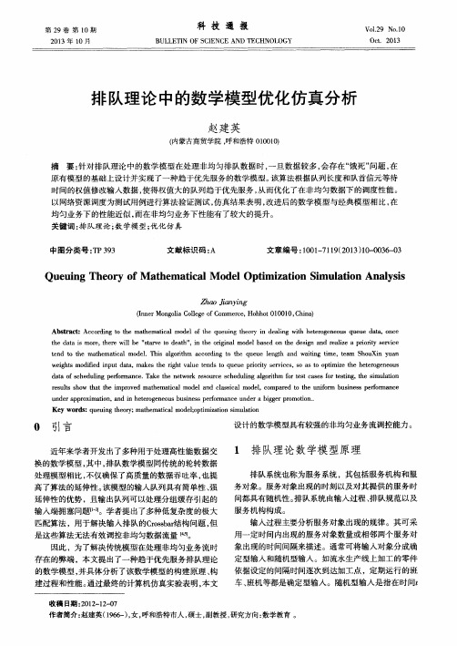
( 内蒙古商贸学院 , 呼和浩 特 0 1 0 0 1 0 ) Nhomakorabea摘
要: 针对 排队理论 中的数学模 型在处理 非均匀排 队数 据时 , 一旦数据 较多 , 会存在 “ 饿 死” 问题 , 在
原有模型 的基础上设计并实现了一种趋 于优先 服务的数学模 型。 该算法根据队列长度和队首信元 等待 时间的权值修改输人数据 , 使得权值大的队列趋于优先 服务 , 从而优化 了在非均匀数据下 的调度性 能。
以网络资源调度 为测试用例进行算法验证测试 , 仿真结 果表明 , 改进后 的数学模型与经典模 型相 比, 在
均匀业务下 的性 能近似 , 而在非均匀业务下性能有 了较大的提升。
关键词 : 排 队理论 ; 数 学模型 ; 优化仿真
中图分类号 : T P 3 9 3
文献标识码 : A
Z h a o J i a n y i n g ( I n n e r M o n g o l i a C o l l e g e o f C o mm e r c e , H o h h o t 0 1 0 0 1 0 , C h i n a )
Ab s t r a c t :Ac c o r d i n g t o t h e ma t h e ma t i c a l mo d e l o f t h e q u e u i n g t h e o r y i n d e li a n g wi h t h e t e r o g e n e o u s q u e u e d a t a ,o n c e
第 2 9卷 第 1 O期
2 0 1 3年 1 O月
科 技 通 报
BU L LE T I N OF S CI ENC E A ND T E CHN0I OGY
基于排队论医院仿真优化研究
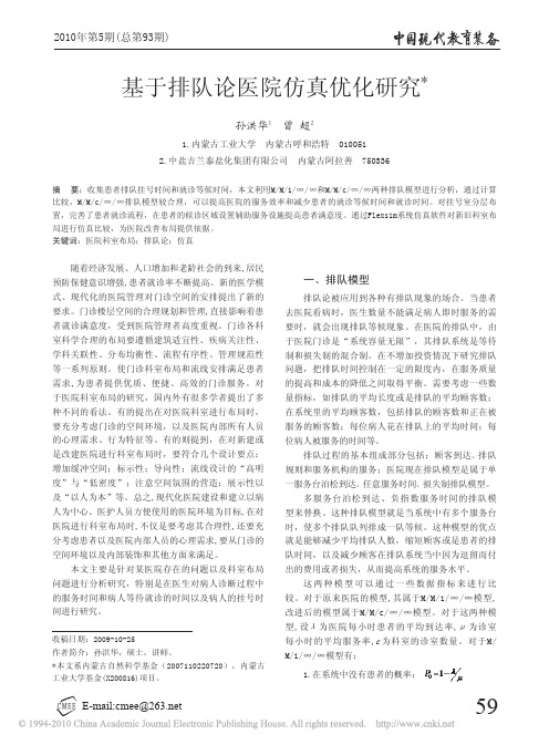
592010年第5期(总第93期)E-基于排队论医院仿真优化研究*孙洪华1 曾 超21.内蒙古工业大学 内蒙古呼和浩特 0100512.中盐吉兰泰盐化集团有限公司 内蒙古阿拉善 750336摘 要:收集患者排队挂号时间和就诊等候时间,本文利用M/M/1/∞/∞和M/M/c/∞/∞两种排队模型进行分析,通过计算比较,M/M/c/∞/∞排队模型较合理,可以提高医院的服务效率和减少患者的就诊等候时间和就诊时间。
对挂号室分层布置,完善了患者就诊流程,在患者的候诊区域设置辅助服务设施提高患者满意度。
通过Flexsim系统仿真软件对新旧科室布局进行仿真比较,为医院改善布局提供依据。
关键词:医院科室布局;排队论;仿真收稿日期:2009-10-25作者简介:孙洪华,硕士,讲师。
*本文系内蒙古自然科学基金(2007110220720),内蒙古工业大学基金(X200816)项目。
随着经济发展、人口增加和老龄社会的到来,居民预防保健意识增强,患者就诊率不断提高。
新的医学模式、现代化的医院管理对门诊空间的安排提出了新的要求。
门诊楼层空间的合理规划和管理,直接影响着患者就诊满意度,受到医院管理者高度重视。
门诊各科室科学合理的布局要遵循建筑适宜性、疾病关注性、学科关联性、分布均衡性、流程有序性、管理规范性等一系列原则。
使门诊科室布局和流线安排满足患者需求,为患者提供优质、便捷、高效的门诊服务。
对于医院科室布局的研究,国内外有很多学者提出了多种不同的看法。
有的提出在对医院科室进行布局时,要充分考虑门诊的空间环境,以及医院内部所有人员的心理需求、行为特征等。
有的则提到,在对新建或是改建医院进行科室布局时,要符合几个设计要点:增加缓冲空间;标示性;导向性;流线设计的“高明度”与“低密度”;注意空间氛围的营造;展示性以及“以人为本”等。
总之,现代化医院建设和建立以病人为中心、医护人员方便使用的医院环境为目标,在对医院进行科室布局时,不仅是要考虑其合理性,还要充分考虑患者以及医院内部人员的心理需求,要从门诊的空间环境以及内部装饰和其他方面来满足。
用Matlab实现排队过程的仿真
用Matlab实现排队过程的仿真一、引言排队是日常生活中经常遇到的现象。
通常,当人、物体或是信息的到达速率大于完成服务的速率时,即出现排队现象。
排队越长,意味着浪费的时间越多,系统的效率也越低。
在日常生活中,经常遇到排队现象,如开车上班、在超市等待结账、工厂中等待加工的工件以及待修的机器等。
总之,排队现象是随处可见的。
排队理论是运作管理中最重要的领域之一,它是计划、工作设计、存货控制及其他一些问题的基础。
Matlab 是MathWorks 公司开发的科学计算软件,它以其强大的计算和绘图功能、大量稳定可靠的算法库、简洁高效的编程语言以及庞大的用户群成为数学计算工具方面的标准,几乎所有的工程计算领域,Matlab 都有相应的软件工具箱。
选用 Matlab 软件正是基于 Matlab 的诸多优点。
二、排队模型三.仿真算法原理( 1 )顾客信息初始化根据到达率λ和服务率µ来确定每个顾客的到达时间间隔和服务时间间隔。
服务间隔时间可以用负指数分布函数 exprnd() 来生成。
由于泊松过程的时间间隔也服从负指数分布,故亦可由此函数生成顾客到达时间间隔。
需要注意的是 exprnd() 的输入参数不是到达率λ和服务率µ而是平均到达时间间隔 1/ λ和平均服务时间 1/ µ。
根据到达时间间隔,确定每个顾客的到达时刻 . 学习过 C 语言的人习惯于使用 FOR 循环来实现数值的累加,但 FOR 循环会引起运算复杂度的增加而在 MATLAB 仿真环境中,提供了一个方便的函数 cumsum() 来实现累加功能读者可以直接引用对当前顾客进行初始化。
第 1 个到达系统的顾客不需要等待就可以直接接受服务其离开时刻等于到达时刻与服务时间之和。
( 2 )进队出队仿真在当前顾客到达时刻,根据系统内已有的顾客数来确定是否接纳该顾客。
若接纳则根据前一顾客的离开时刻来确定当前顾客的等待时间、离开时间和标志位;若拒绝,则标志位置为 0。
基于排队论的港口服务系统的建模与仿真研究

基于排队论的港口泊位系统的建模与仿真研究摘要:本文总结了排队论和仿真技术的发展以及应用情况,在前人的研究基础之上分析了系统仿真技术在港口泊位系统中的应用。
分析了研究港口系统服务的特征,建立了港口运营生产的计算机仿真系统,系统充分考虑了港口生产的随机特性及其影响因素,能够比较客观地反映港口的实际运行状况,获得可靠的港口数值特征值,为综合性港口的优化设计提供了参考数据。
本文还结合实例分析,研究探讨了港口泊位利用率和锚地保证率,借助计算机仿真技术、排队论方法构造泊位服务系统模拟模型和分析泊位服务水平,具有一定的实际指导意义。
前言加入WTO以后,我国对外贸易事业得到迅猛发展,港口业也进入了快速增长时期,港口吞吐量逐年上升。
日益增长的吞吐量需求给我国能力不足的港口业既带来了发展机遇,也带来了巨大的挑战。
如何满足巨大的船舶吞吐量需求,提高码头作业效率,降低运作成本,成为了港口业亟待解决的重要课题。
排队论发展及其应用排队论是在概率论和数理统计基础上发展起来的运筹学分支,它是解决排队问题的有效手段。
排队系统的数学研究开始于1909~1920年之间,丹麦工程师爱尔朗(AzKzErlang)在电话交换机的设计上为解决等线和通道问题首先提出了最初的排队论方法,1928年福瑞(Fry)在这个领域做出了较大贡献,促进了排队论的早期研究工作。
50年代初肯德尔(DZGZKendall)对排队论的研究代表了当时该领域的研究水平,他提出的肯德尔符号一直沿用到今天,并依此对排队模型进行分类。
在日常生活及工程中,排队现象无处不在、无时不有。
例如,顾客去商店购买商品、顾客去服务场所接受某种服务(理发、就餐等)、机械零件在车间中加工、运输车辆由装载机装料、船舶进港靠泊码头等,当不能立即得到服务时就需要等待服务(若允许排队等待),因而就发生了排队现象。
排队现象的产生主要是由于要求服务者的到达是随机的,服务机构的服务时间也是随机的,在某时刻要求服务者的数量超过了服务机构的容量,服务者就需要排队等待。
基于Arena的影印店排队系统仿真建模与学习资料
摘要影印店是大学校园里一种很重要的配套设备,而影音店排长队现象是困扰店家和客户的一大难题,减少客户的等候时间,提高商铺的服务效率,成为关注的焦点。
Arena 仿真技术能对这类复杂排队系统进行实质模拟从而对其优化。
本文用 Arena仿真软件剖析确立客户抵达间隔的散布和办理时间的散布,并用假定查验方法进行查验,确立散布种类,最后模拟一个影音店的工作过程,依据实体排队间隔时间等指标,提高影音店的运转效率。
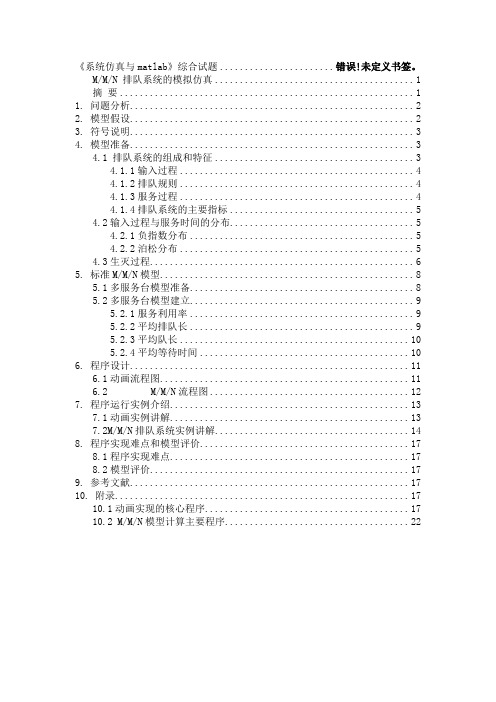
重点字: Arena,仿真,影印店,排队一、前言 (2)二、原理简述 (2)三、实地调研及数据采集 (3)四、数据剖析办理 (3)4.1 客人到店的时间间隔 (3)4.2 打印的服务时间 (4)4.3 复印的服务时间 (4)五、模型成立 (5)5.1 客户抵达模块 (5)5.2 选择服务模块 (5)5.3 接受服务模块 (5)5.3.1 打印服务模块 (6)5.3.2 复印服务模块 (6)5.4 走开模块 (7)5.5模型整体构造图 (7)六、仿真 (7)6.1 仿真运转参数 (7)6.2 仿真结果剖析 (8)七、优化及结果剖析 (9)7.1 延伸服务时间 (9)7.2 增添机器数目 (10)八、结论 (11)参照文件 (11)一、前言今世学生不论在考试仍是平常,都会用到试卷和各样资料。
此刻不是每种资料都要去书店买,有的资料在书店也买不到,有些不过需要参照书中的一部分,那么买整本书就很不合实质,此时就需要复印。
方便 ,快捷 ,也能够节俭不用要的开销。
今世大学生特别需要这样的服务。
在考试前夜,老师会总结一些实用的复习资料供应给大家作为参照,这类资料常常是以电子邮件的形式发放,各高校的学生其实不都是当地学生,所以只有益用影印店,即便是当地学生,大多数为了方便也都会选择学校邻近的影印店来解决资料问题。
顾客增加,要减少排队等候时间就要增添机器数目,就要增添营业成本;而增添机器数目有可能出现安闲,又浪费资源。
所以,怎样找到一个均衡点,使三者达到最正确的均衡状态,是解决影印店排队问题的重点。
基于Matlab的排队问题仿真
自 10 9 9年 E L N R A G开创 性 的论 文 发表 以 来 , 队论 理 论 广 泛 应 用 于通 信 、 事 、 输 、 排 军 运 维
第3 卷 第 6 2 期
21 00年 1 2月
武 汉 理 工 大 学 学 报 ・信 息 与 管 理 工 程 版
J U N L O T I F R TO O R A FWU (N O MA IN& M N G ME TE G N E IG) A A E N N IE R N
Vo _ 2 . l3 No 6 De 2 0 c. 01
应结果 。
统 内有 n个 顾客 的概 率 P () t满足 方程 :
收稿 日期 :00— 6— 2 21 0 2.
作者简介: 李字光 (9 6一) 男 , 16 , 湖北天 门人 , 武汉理工大学理学 院讲师
第3 2卷
第 6期
李 宇光 : 基于 M t b的排队问题仿真 aa l
而某 阶段 服务员 又空 闲无 事 的情 形 。服务 系统 的 服务 能力一 方 面取决 于服 务员 的数量 和服 务员 的 能力 ; 另一 方 面也 取 决 于 顾 客 流 的性 质 。排 队 问 题就 是要 寻求顾 客流 、 务 能 力 和 服务 系统 效益 服
足 这种假 设 , 因此 需要 有更 一般 的方法 。
理 包括 线性 、 非线 性 系统 、 离散 、 连续 及混 合 、 任 单
基于排队论和整数规划的银行柜员弹性排班模型

基于排队论和整数规划的银行柜员弹性排班模型一、本文概述随着银行业务的日益发展和客户需求的多样化,银行柜员排班问题成为了银行业务运营中的关键环节。
传统的固定排班模式已难以满足现代银行业务的需求,因此,开发一种基于排队论和整数规划的银行柜员弹性排班模型显得尤为重要。
本文旨在探讨如何运用排队论和整数规划的理论和方法,构建一个既能满足客户需求,又能保证柜员工作效率和满意度的弹性排班模型。
排队论作为一种研究服务系统中排队现象的数学工具,可以分析客户到达和服务的统计规律,为银行柜员排班提供理论基础。
整数规划则是一种求解最优化问题的数学方法,通过约束条件和目标函数的设置,可以求得满足实际需求的柜员排班方案。
本文将首先介绍排队论和整数规划的基本原理及其在银行柜员排班中的应用背景,然后详细阐述基于排队论和整数规划的银行柜员弹性排班模型的构建过程,包括模型的假设、参数设定、约束条件构建以及目标函数的确定。
通过实例分析验证模型的有效性和实用性,并提出模型的改进方向和应用前景。
本文的研究不仅有助于提升银行柜员排班的科学性和合理性,还可以为银行业务的持续优化和客户服务质量的提升提供有力支持。
也为其他服务行业在弹性排班模型的构建和应用方面提供有益的参考和借鉴。
二、理论基础本研究所构建的银行柜员弹性排班模型主要基于两个理论基础:排队论和整数规划。
这两个理论在运筹学、管理科学和工程领域具有广泛的应用,尤其在处理资源优化配置和服务系统效率提升的问题上表现出色。
排队论,又称为随机服务系统理论,主要研究服务系统中等待队列的形成、发展和变化规律,以及系统的性能特征。
在银行柜员排班问题中,客户到达银行办理业务的过程就是一个典型的排队过程。
排队论中的关键概念包括顾客到达率、服务率等待时间、队列长度等,这些指标直接影响到银行的服务质量和顾客满意度。
通过排队论,我们可以对银行柜员的工作强度、服务效率以及顾客等待时间进行数学建模,为合理的排班安排提供理论支持。
排队论系统仿真

于零,即
dPn (t ) 0, 对一切n 。 dt 因为稳态和时间无关,所以将符号简化,用 Pn 代替 Pn(t),于是
Pn n 1 n 2 0 P0 n n 1 1
i 0 n i 1
——平均服务率,即单位时间内接受服务的顾客数;
C——并列服务台的个数;
——服务强度。
通常,排队论研究的相关问题可大体分成统计问题和最优化问题两大类。 统计问题是排队系统建模中的一个组成部分,它主要研究对现实数据的处理 问题, 在输入数据的基础上, 首先要研究顾客相继到达的间隔时间是否独立同分
布,如果是独立同分布,还要研究分布类型以及有关参数的确定问题.类似地, 对服务时间也要进行相应的研究。 排队系统的优化问题涉及到系统的设计、控制以及有效性评价等方面的内 容。 排队论本身不是一种最优化方法,它是一种分析工具。常见的系统最优设计 问题是在系统设置之前, 根据已有的顾客输入与服务过程等资料对系统的前景进 行估计或预测,依此确定系统的参数。 系统最优控制问题是根据顾客输入的变化而对现有服务系统进行的适度调 整,即根据系统的实际情形,制定一个合理的控制策略,并据此确定系统运行的 最佳参数。作为一种分析工具,处理排队问题的过程可以概括为以下四步: (1)确定排队问题的各个变量,建立它们之间的相互关系; (2)根据已知的统计数据, 运用适当的统计检验方法以确定相关的概率分布; (3)根据所得到的概率分布,确定整个系统的运行特征; (4)根据服务系统的运行特征,按照一定的目的,改进系统的功能。
P0 (t ) e t
T 小于等于 t 的概率 P(T≤t)表示为 F(t) (累积分布函数) ,有
F (t ) 1 et
剖析超市排队的仿真模型应用论文

剖析超市排队的仿真模型应用论文论文关键词:动态模拟;蒙特卡洛模拟;排队论论文内容摘要:综合考虑顾客等待成本和商场的成本效益,进而得出超市为满足一定服务水平应该开设的服务器个数。
本文根据超市顾客到达的随机性和服务时间的随机性,用蒙特卡洛方法模拟不同的顾客到达和服务水平,在MATLAB/Simulink上对超市单队列多收银台的服务系统进行了动态模拟仿真,得到不同顾客到达率和不同服务水平下,顾客的排队等待时间,服务器的空闲率等要素。
在超市收银排队系统中,顾客希望排队等待的时间越短越好,这就需要服务机构设置较多的收银台,这样可以减少排队等待时间,但会增加商场的运营成本。
而收银台过少,会使服务质量降低,甚至造成顾客流失。
如何科学合理地设置收银台的数量,以降低成本和提高效益,是商场管理人员需要解决的一个重要问题。
蒙特卡洛方法简介蒙特卡洛方法又称随机模拟方法,它以随机模拟和统计试验为手段,从符合某种概率分布的随机变量中,通过随机选择数字的方法,产生一组符合该随机变量概率分布特性的随机数值序列,作为输入变量序列进行特定的模拟试验、求解(杜比,2007)。
在应用该方法时,步骤1:建立概率模型,即将所研究的问题变为概率问题,构造一个符合其特点的概率模型;步骤2:产生一组符合该随机变量概率分布特性的随机数值序列;步骤3:以随机数值序列作为系统的抽样输入进行大量的数字模拟试验,以得到模拟试验值;步骤4:对模拟试验结果进行统计处理(如计算频率、均值等),进而对研究问题做出解释。
基于排队理论的仿真模型建立(一)超市服务排队模型(M/M/C)超市收款台服务是一个随机服务系统(唐应辉,2006),该系统具有如下特征:服务的对象是已经选购好商品的顾客,顾客源是无限的,顾客之间相互独立,顾客相继到达的时间间隔是随机的。
系统有多个服务员且对每个顾客的服务时间是相互独立的。
服务规则遵从先到后服务(FCFS)的原则。
每个收款台前都有排队队列,顾客选择较短的队列排队等候,这样形成单队列多服务员(M/M/C)的排队系统。
基于Matlab的排队问题仿真

f ( S ) =β1 e- S /βS ( S ≥0) S
应用反变换法 [2 ] ,得
A
=
-
β A
ln u1 S
=
-
β S
ln u2
其中 , u1 , u2 为 U ( 0, 1)分布随机数 。
1. 2 建立事件表
由于采用面向事件的仿真方法 , 仿真钟按下一
个最早发生事件的发生时间推进 。由此对引起系统
(上接第 14页 )
4 结束语
采用超临界 CO2 萃取大豆磷脂工艺简单 ,设备 单一 ,无溶剂残留等优点 ,所用溶剂 CO2 的性质稳 定 ,安全 ,操作方便 ,耗能低 ,价格便宜 ,提取成本较 低 。所以 ,超临界 CO2 萃取法比其它方法更优越 。 对超临界 CO2 流体萃取大豆磷脂的精制方法进行 的初步研究 ,可做以下确定 。 4. 1 超临界 CO2 萃取技术可有效地提高大豆磷脂 的含量 ,其纯度可达到 95%以上 。 4. 2 由于磷脂不溶于超临界 CO2 和乙醇 ,因此在
高静涛 , 史百战
(兰州交通大学 机电技术研究所 ,甘肃 兰州 730070)
摘 要 : 排队问题仿真的目的 ,就是要寻找服务对象与服务设置之间的最佳配置 ,保证系统具 有最佳的服务效率与最合理的配置 。本文讨论了排队问题的基本要素 ,并提出一套标准的求 解公式 。通过 M atlab软件对这些公式的仿真 ,来协助计划人员分析顾客的需求 ,从而建立符 合现有条件的服务设施 。 关键词 : M atlab; 排队问题 ; 仿真 中图分类号 : TP 39119; O 226 文献标识码 : A
Q ( t) ———t时刻排队等待的顾客数 ; T———完成 n个
顾客服务所需时间 。
排队论模型与蒙特卡罗仿真

P{x(tn ) n |x(t1 )x1 ,x(t2 )x2 ,...,x(tn1 )xn1 } P{x(tn ) n |x(tn1 )xn1 }
也就是说过程在t+Δ t所处的状态与t以前所处的状 态无关。 ②平稳性:即对于足够小的Δ t,有:
P1 ( t,t t ) t ( t )
在[t,t+Δ t]内有一个顾客到达的概率与t无关, 26 而与Δ t成正比。
λ >0 是常数,它表示单位时间到达的顾客数,称 为概率强度。 ③ 普通性:对充分小的 Δ t,在时间区间(t,t+Δ t) 内有2个或2个以上顾客到达的概率是一高阶无穷小. 即
Pn (t , t t ) o(t )
排队可以是有形的,也可以是无形的。 如几个顾客打电话到出租车站要车,如 果出租车站无足够车辆,则部分顾客只得在 要车处等待,他们分散在不同地方,形成一 个无形的排队序列。
5
排队的不一定是人,也可以是物。 例如:生产线上等待加工的原料、半 成品; 因故障停止运转等待修理的机器等。
6
上述问题虽互不相同,但却都有 要求得到某种服务的人或物以及提供 服务的人或机构。 排队论里把要求服务的对象统称 为“顾客” , 提供服务的人或机构称 为“服务台”或“服务员”。
13
3 . 1 . 2. 排队规则
分为损失制、等待制、混合制三大类。 (1) 损失制 指如果顾客到达排队系统 时,所有服务台都已被先来的顾客占用, 那么他们就自动离开系统永不再来。 典型例子是,如电话拔号后出现忙音, 顾客不愿等待而自动挂断电话,如要再打, 就需重新拔号。
14
(2) 等待制 当顾客来到系统时,所有服务台都 不空,顾客加入排队行列等待服务。 例如,排队等待售票,故障设备等待维修等。 等待制中,服务台在选择顾客进行服务时,常有 如下四种规则:
MMN排队系统建模与仿真
《系统仿真与matlab》综合试题....................... 错误!未定义书签。
M/M/N 排队系统的模拟仿真 (1)摘要 (1)1. 问题分析 (2)2. 模型假设 (2)3. 符号说明 (3)4. 模型准备 (3)4.1 排队系统的组成和特征 (3)4.1.1输入过程 (4)4.1.2排队规则 (4)4.1.3服务过程 (4)4.1.4排队系统的主要指标 (5)4.2输入过程与服务时间的分布 (5)4.2.1负指数分布 (5)4.2.2泊松分布 (5)4.3生灭过程 (6)5. 标准M/M/N模型 (8)5.1多服务台模型准备 (8)5.2多服务台模型建立 (9)5.2.1服务利用率 (9)5.2.2平均排队长 (9)5.2.3平均队长 (10)5.2.4平均等待时间 (10)6. 程序设计 (11)6.1动画流程图 (11)6.2 M/M/N流程图 (12)7. 程序运行实例介绍 (13)7.1动画实例讲解 (13)7.2M/M/N排队系统实例讲解 (14)8. 程序实现难点和模型评价 (17)8.1程序实现难点 (17)8.2模型评价 (17)9. 参考文献 (17)10. 附录 (17)10.1动画实现的核心程序 (17)10.2 M/M/N模型计算主要程序 (22)M/M/N 排队系统的模拟仿真摘要排队是在日常生活中经常遇到的事,由于顾客到达和服务时间的随机性,使得排队不可避免。
因此,本文建立标准的M/M/N模型,并运用Matlab软件,对M/M/N排队系统就行了仿真,从而更好地深入研究排队问题。
问题一,基于顾客到达时间服从泊松分布和服务时间服从负指数分布,建立了标准的M/M/N模型。
运用Matlab软件编程,通过输入服务台数量、泊松分布参数以及负指数分布参数,求解出平均队长、服务利用率、平均等待时间以及平均排队长等重要指标。
然后,分析了输入参数与输出结果之间的关系。
- 1、下载文档前请自行甄别文档内容的完整性,平台不提供额外的编辑、内容补充、找答案等附加服务。
- 2、"仅部分预览"的文档,不可在线预览部分如存在完整性等问题,可反馈申请退款(可完整预览的文档不适用该条件!)。
- 3、如文档侵犯您的权益,请联系客服反馈,我们会尽快为您处理(人工客服工作时间:9:00-18:30)。
关键词:动态模拟蒙特卡洛模拟排队论
内容摘要:论文根据超市顾客到达的随机性和服务时间的随机性,用蒙特卡洛方法模拟不同的顾客到达和服务水平,在MA TLAB/Simulink上对超市单队列多收银台的服务系统进行了动态模拟仿真,得到不同顾客到达率和不同服务水平下,顾客的排队等待时间,服务器的空闲率等要素。
在超市收银排队系统中,顾客希望排队等待的时间越短越好,这就需要服务机构设置较多的收银台,这样可以减少排队等待时间,但会增加商场的运营成本。
而收银台过少,会使服务质量降低,甚至造成顾客流失。
如何科学合理地设置收银台的数量,以降低成本和提高效益,是商场管理人员需要解决的一个重要问题。
蒙特卡洛方法简介
蒙特卡洛方法又称随机模拟方法,它以随机模拟和统计试验为手段,从符合某种概率分布的随机变量中,通过随机选择数字的方法,产生一组符合该随机变量概率分布特性的随机数值序列,作为输入变量序列进行特定的模拟试验、求解(杜比,2007)。
在应用该方法时,要求产生的随机数序列应符合该随机变量特定的概率分布。
应用该方法的基本步骤如下:
步骤1:建立概率模型,即将所研究的问题变为概率问题,构造一个符合其特点的概率模型;步骤2:产生一组符合该随机变量概率分布特性的随机数值序列;步骤3:以随机数值序列作为系统的抽样输入进行大量的数字模拟试验,以得到模拟试验值;步骤4:对模拟试验结果进行统计处理(如计算频率、均值等),进而对研究问题做出解释。
基于排队理论的仿真模型建立
(一)超市服务排队模型(M/M/C)
超市收款台服务是一个随机服务系统(唐应辉,2006),该系统具有如下特征:服务的对象是已经选购好商品的顾客,顾客源是无限的,顾客之间相互独立,顾客相继到达的时间间隔是随机的。
系统有多个服务员且对每个顾客的服务时间是相互独立的。
服务规则遵从先到后服务(FCFS)的原则。
每个收款台前都有排队队列,顾客选择较短的队列排队等候,这样形成单队列多服务员(M/M/C)的排队系统。
超市收银台顾客排队系统结构见图1。
(二)产生随机数值序列
由于顾客到达间隔时间和顾客服务的时间服从负指数颁布的随机数。
令这个负指数分布的随机数为x,负指数分布密度函数为:,其分布函数为:,F(x)的反函数为。
设u为[0,1]区间上的独立、均匀分布的随机变量,则所求随机数为,进而简化得,这样得到负指数分布的随机数(吴飞,2006)。
针对商场顾客到达和服务水平的统计数据,据此可产生两个随机数列:顾客到达时间间隔a (i)和顾客服务时间st(i),以此数值序列进行动态输入仿真。
(三)模型变量设置
at(i):表示第i
个顾客到达时刻;
a(i):表示第i个顾客到达的时间间隔;st(i):第i个顾客的服务时间;sst(i):
第i个顾客的开始服务时间;lea(i):第i个顾客离开时间;ls(j):第j个队列中最后一个顾客的离开时间;ls(m):每个队列中最后一个顾客离开时间的最早值;freet(j):第j个
服务员的平均空闲时间;w(i):第i个顾客进入系统后的排队等待时间。
其中:at(i+1)=at(i)+a(i+1),sst(i)=max(at(i),ls(m)),w(i)=max(0,ls(m)-at(i)),ls(m)=min(lt(j))。
仿真系统模拟
(一)超市收银台服务仿真模拟
解决超市收银台顾客排队问题,关键是要测量常态下需要多少收银台才是适宜的。
根据商场收银台服务统计数据,可以测算出超市收银员的服务率、顾客到达率,
然后通过仿真方法测量出超市提供多少收银台才最适宜。
基本步骤如下:
系统经过较长时间运行后达到平稳。
根据实际考察,一周之内,双休日及节假日的客流量剧增,而在一天之中顾客的到达也出现几个高峰期,所以,作如下改进:将一天分为四个时段(9:00-12:00,12:00-14:00,14:00-18:00,18:00-21:00),首先调查其中一个时段(以第三时段为例)周一至周五的工作状况,调查数据如表1所示。
根据统计数据得到了单位时间内到达的顾客数n和为每位顾客服务的时间t,然后利用χ2拟合检验(包科研、李娜,2008),得到单位时间的顾客到达数服从Possion分布,服务时间服从负指数分布。
根据资料统计得到单服务台服务强度为每小时49人,即μ=49,到达速率每小时277人,即λ=277。
设定顾客平均等待时间小于5分钟,模拟次数1000次,模拟超市应设置多少收银台。
同时,这里的μ和λ可以根据不同时段的实际情况变化,以模拟在不同到达速率和服务强度下的工作状态。
(二)仿真程序设计
首先顾客按规定的到达模式产生到达,同时按规定的服务模式产生服务时间,然后判断是否有空闲的服务台。
有,则直接接受服务而不需进入队列等待;否则,顾客将进入队列等待服务。
顾客选择等待服务台队列时,以最早接受服务为标准,此前要计算各服务台进入空闲的时间。
仿真钟采用事件调度法,以顾客到达为驱动。
一个顾客进入系统后,按仿真方法和流程计算其服务时间与离开时间后,驱动下一个事件(下一个顾客的到达)的发生。
在仿真过程中还要对服务台利用率、队列长度、顾客等待时间等进行统计以达到仿真目的,如图2所示。
该模型(M/M/C)以第三时段为例,顾客随机性到达,到达模式服从泊松分布λ=277;服务时间也是随机的,服从指数分布,每小时服务人数为μ=49;纪录到2000名顾客时模拟终止,仿真采用基于事件(基于顾客)的方法。
本文以MA TLAB7.0/Simulink6.0仿真系统为工具进行动态模拟仿真(黄永安,2007),仿真次数1000次,结果取平均值。
参考文献:
1.杜比.蒙特卡洛方法在系统工程中的应用[M].西安交通大学出版社,2007
2.唐应辉.排队论[M].科学出版社,2006
3.吴飞.产生随机数的几种方法及应用[J].数值计算与计算机应用,2006.3
4.包科研,李娜.数理统计与MA TLAB数据处理[M].东北大学出版社,2008。