弹性力学双语讲义(Chapter3)
chapter_3

3Stress and EquilibriumThe previous chapter investigated the kinematics of deformation without regard to the force orstress distribution within the elastic solid.We now wish to examine these issues and explorethe transmission of forces through deformable materials.Our study leads to the definition anduse of the traction vector and stress tensor.Each provides a quantitative method to describeboth boundary and internal force distributions within a continuum solid.Because it is com-monly accepted that maximum stresses are a major contributing factor to material failure,primary application of elasticity theory is used to determine the distribution of stress within agiven structure.Related to these force distribution issues is the concept of equilibrium.Withina deformable solid,the force distribution at each point must be balanced.For the static case,the summation of forces on an infinitesimal element is required to be zero,while for a dynamicproblem the resultant force must equal the mass times the element’s acceleration.In thischapter,we establish the definitions and properties of the traction vector and stress tensor anddevelop the equilibrium equations,which become another set offield equations necessary inthe overall formulation of elasticity theory.It should be noted that the developments in thischapter do not require that the material be elastic,and thus in principle these results apply to abroader class of material behavior.3.1Body and Surface ForcesWhen a structure is subjected to applied external loadings,internal forces are inducedinside the body.Following the philosophy of continuum mechanics,these internal forces aredistributed continuously within the solid.In order to study such forces,it is convenient tocategorize them into two major groups,commonly referred to as body forces and surfaceforces.Body forces are proportional to the body’s mass and are reacted with an agent outside of the body.Examples of these include gravitational-weight forces,magnetic forces,and inertialforces.Figure3-1(a)shows an example body force of an object’s self-weight.By usingcontinuum mechanics principles,a body force density(force per unit volume)F(x)can bedefined such that the total resultant body force of an entire solid can be written as a volumeintegral over the body49F R ¼ðððV F (x )dV (3:1:1)Surface forces always act on a surface and result from physical contact with another body.Figure 3-1(b)illustrates surface forces existing in a beam section that has been created by sectioning the body into two pieces.For this particular case,the surface S is a virtual one in the sense that it was artificially created to investigate the nature of the internal forces at this location in the body.Again the resultant surface force over the entire surface S can be expressed as the integral of a surface force density function T n (x )F S ¼ððS T n (x )dS (3:1:2)The surface force density is normally referred to as the traction vector and is discussed in more detail in the next section.In the development of classical elasticity,distributions of body or surface couples are normally not included.Theories that consider such force distributions have been constructed in an effort to extend classical elasticity for applications in micromechanical modeling.Such approaches are normally called micropolar or couple-stress theory (see Eringen 1968)and are briefly presented in Chapter14.(b) Sectioned Axially Loaded BeamT(x)(a) Cantilever Beam Under Self-Weight LoadingFIGURE 3-1Examples of body and surface forces.50FOUNDATIONS AND ELEMENTARY APPLICATIONS3.2Traction Vector and Stress TensorIn order to quantify the nature of the internal distribution of forces within a continuum solid,consider a general body subject to arbitrary(concentrated and distributed)external loadings,asshown in Figure3-2.To investigate the internal forces,a section is made through the body asshown.On this section consider a small area D A with unit normal vector n.The resultantsurface force acting on D A is defined by D F.Consistent with our earlier discussion,noresultant surface couple is included.The stress or traction vector is defined byT n(x,n)¼limD A!0D FD A(3:2:1)Notice that the traction vector depends on both the spatial location and the unit normal vector to the surface under study.Thus,even though we may be investigating the same point,the traction vector still varies as a function of the orientation of the surface normal.Because the traction is defined as force per unit area,the total surface force is determined through integration as per relation(3.1.2).Note,also,the simple action-reaction principle(Newton’s third law)T n(x,n)¼ÀT n(x,Àn)Consider now the special case in which D A coincides with each of the three coordinate planes with the unit normal vectors pointing along the positive coordinate axes.This concept is shown in Figure3-3,where the three coordinate surfaces for D A partition off a cube of material.For this case,the traction vector on each face can be written asT n(x,n¼e1)¼s x e1þt xy e2þt xz e3T n(x,n¼e2)¼t yx e1þs y e2þt yz e3T n(x,n¼e3)¼t zx e1þt zy e2þs z e3(3:2:2)where e1,e2,e3are the unit vectors along each coordinate direction,and the nine quantities {s x,s y,s z,t xy,t yx,t yz,t zy,t zx,t xz}are the components of the traction vector on each of three coordinate planes as illustrated.These nine components are called the stress components,(Sectioned Body)FIGURE3-2Sectioned solid under external loading.Stress and Equilibrium51with s x ,s y ,s z referred to as normal stresses and t xy ,t yx ,t yz ,t zy ,t zx ,t xz called the shear-ing stresses .The components of stress s ij are commonly written in matrix formats ¼[s ]¼s xt xy t xz t yxs y t yz t zx t zy s z 2435(3:2:3)and it can be formally shown that the stress is a second-order tensor that obeys the appropriate transformation law (1:5:3)3.The positive directions of each stress component are illustrated in Figure 3-3.Regardless of the coordinate system,positive normal stress always acts in tension out of the face,and only one subscript is necessary because it always acts normal to the surface.The shear stress,however,requires two subscripts,the first representing the plane of action and the second designating the direction of the stress.Similar to shear strain,the sign of the shear stress depends on coordinate system orientation.For example,on a plane with a normal in the positive x direction,positive t xy acts in the positive y direction.Similar definitions follow for the other shear stress components.In subsequent chapters,proper formulation of elasticity problems requires knowledge of these basic definitions,directions,and sign conventions for particular stress components.Consider next the traction vector on an oblique plane with arbitrary orientation,as shown in Figure 3-4.The unit normal to the surface can be expressed byn ¼n x e 1þn y e 2þn z e 3(3:2:3)where n x ,n y ,n z are the direction cosines of the unit vector n relative to the given coordinate system.We now consider the equilibrium of the pyramidal element interior to the oblique and coordinate planes.Invoking the force balance between tractions on the oblique and coordinate faces givess ys xFIGURE 3-3Components of the stress.52FOUNDATIONS AND ELEMENTARY APPLICATIONST n ¼n x T n (n ¼e 1)þn y T n (n ¼e 2)þn z T n (n ¼e 3)and by using relations (3.2.2),this can be written asT n ¼(s x n x þt yx n y þt zx n z )e 1þ(t xy n x þs y n y þt zy n z )e 2þ(t xz n x þt yz n y þs z n z )e 3(3:2:4)or in index notationT n i ¼s ji n j (3:2:5)Relation (3.2.4)or (3.2.5)provides a simple and direct method to calculate the forces on oblique planes and surfaces.This technique proves to be very useful to specify general boundary conditions during the formulation and solution of elasticity problems.Following the principles of small deformation theory,the previous definitions for the stress tensor and traction vector do not make a distinction between the deformed and un-deformed configurations of the body.As mentioned in the previous chapter,such a distinction only leads to small modifications that are considered higher-order effects and are normally neglected.However,for large deformation theory,sizeable differences exist between these configurations,and the undeformed configuration (commonly called the reference configuration)is often used in problem formulation.This gives rise to the definition of an additional stress called the Piola-Kirchhoff stress tensor that represents the force per unit area in the reference configuration (see Chandrasekharaiah and Debnath 1994).In the more general scheme,the stress s ij is referred to as the Cauchy stress tensor.Throughout the text only small deformation theory is considered,and thus the distinction between these two definitions of stress disappears,thereby eliminating any need for this additional terminology.FIGURE 3-4Traction on an oblique plane.Stress and Equilibrium 533.3Stress TransformationAnalogous to our previous discussion with the strain tensor,the stress components must alsofollow the standard transformation rules for second-order tensors established in Section1.5.Applying transformation relation(1.5.1)3for the stress givess0ij¼Q ip Q jq s pq(3:3:1)where the rotation matrix Q ij¼cos(x0i,x j).Therefore,given the stress in one coordinatesystem,we can determine the new components in any other rotated system.For the generalthree-dimensional case,the rotation matrix may be chosen in the formQ ij¼l1m1n1l2m2n2l3m3n32435(3:3:2)Using this notational scheme,the specific transformation relations for the stress then becomes0x¼s x l21þs y m21þs z n21þ2(t xy l1m1þt yz m1n1þt zx n1l1)s0y¼s x l22þs y m22þs z n22þ2(t xy l2m2þt yz m2n2þt zx n2l2)s0z¼s x l23þs y m23þs z n23þ2(t xy l3m3þt yz m3n3þt zx n3l3)t0xy¼s x l1l2þs y m1m2þs z n1n2þt xy(l1m2þm1l2)þt yz(m1n2þn1m2)þt zx(n1l2þl1n2)t0yz¼s x l2l3þs y m2m3þs z n2n3þt xy(l2m3þm2l3)þt yz(m2n3þn2m3)þt zx(n2l3þl2n3) t0zx¼s x l3l1þs y m3m1þs z n3n1þt xy(l3m1þm3l1)þt yz(m3n1þn3m1)þt zx(n3l1þl3n1)(3:3:3)For the two-dimensional case originally shown in Figure2-6,the transformation matrix was given by relation(2.3.4).Under this transformation,the in-plane stress components transform according tos0x¼s x cos2yþs y sin2yþ2t xy sin y cos ys0y¼s x sin2yþs y cos2yÀ2t xy sin y cos yt0 xy ¼Às x sin y cos yþs y sin y cos yþt xy(cos2yÀsin2y)(3:3:4)which is commonly rewritten in terms of the double angles0 x ¼s xþs y2þs xÀs y2cos2yþt xy sin2ys0 y ¼s xþs y2Às xÀs y2cos2yÀt xy sin2yt0 xy ¼s yÀs x2sin2yþt xy cos2y(3:3:5)Similar to our discussion on strain in the previous chapter,relations(3.3.5)can be directlyapplied to establish stress transformations between Cartesian and polar coordinate systems(see Exercise3-3).Both two-and three-dimensional stress transformation equations can be 54FOUNDATIONS AND ELEMENTARY APPLICATIONSeasily incorporated in MATLAB to provide numerical solution to problems of interest(seeExercise3-2).3.4Principal StressesWe can again use the previous developments from Section1.6to discuss the issues of principalstresses and directions.It is shown later in the chapter that the stress is a symmetric tensor.Using this fact,appropriate theory has been developed to identify and determine principal axesand values for the stress.For any given stress tensor we can establish the principal valueproblem and solve the characteristic equation to explicitly determine the principal values anddirections.The general characteristic equation for the stress tensor becomesdet[s ijÀsd ij]¼Às3þI1s2ÀI2sþI3¼0(3:4:1) where s are the principal stresses and the fundamental invariants of the stress tensor can beexpressed in terms of the three principal stresses s1,s2,s3asI1¼s1þs2þs3I2¼s1s2þs2s3þs3s1I3¼s1s2s3(3:4:2) In the principal coordinate system,the stress matrix takes the special diagonal forms ij¼s1000s2000s32435(3:4:3)A comparison of the general and principal stress states is shown in Figure3-5.Notice that for the principal coordinate system,all shearing stresses vanish and thus the state includes only normal stresses.These issues should be compared to the equivalent comments made for the strain tensor at the end of Section2.4.(General Coordinate System)(Principal Coordinate System)FIGURE3-5Comparison of general and principal stress states.Stress and Equilibrium55We now wish to go back to investigate another issue related to stress and traction transformation that makes use of principal stresses.Consider the general traction vector T n that acts on an arbitrary surface as shown in Figure 3-6.The issue of interest is to determine the traction vector’s normal and shear components N and S .The normal component is simply the traction’s projection in the direction of the unit normal vector n ,while the shear component is found by Pythagorean theorem,N ¼T n ÁnS ¼(j T n j 2ÀN 2)1=2(3:4:4)Using the relationship for the traction vector (3.2.5)into (3:4:4)1givesN ¼T n Án ¼T n i n i ¼s ji n j n i¼s 1n 21þs 2n 22þs 3n 23(3:4:5)where,in order to simplify the expressions,we have used the principal axes for the stress tensor.In a similar manner,j T n j 2¼T n ÁT n ¼T n i T n i ¼s ji n j s ki n k¼s 21n 21þs 22n 22þs 23n 23(3:4:6)Using these results back into relation (3.4.4)yieldsN ¼s 1n 21þs 2n 22þs 3n 23S 2þN 2¼s 21n 21þs 22n 22þs 23n 23(3:4:7)In addition,we also add the condition that the vector n has unit magnitude1¼n 21þn 22þn 23(3:4:8)Relations (3.4.7)and (3.4.8)can be viewed as three linear algebraic equations for theunknowns n 21,n 22,n 23.Solving this system gives the following result:T nFIGURE 3-6Traction vector decomposition.56FOUNDATIONS AND ELEMENTARY APPLICATIONSn21¼S2þ(NÀs2)(NÀs3) (s1Às2)(s1Às3)n22¼S2þ(NÀs3)(NÀs1) (s2Às3)(s2Às1)n23¼S2þ(NÀs1)(NÀs2)(s3Às1)(s3Às2)(3:4:9)Without loss in generality,we can rank the principal stresses as s1>s2>s3.Noting that the expressions given by(3.4.9)must be greater than or equal to zero,we can conclude the followingS2þ(NÀs2)(NÀs3)!0S2þ(NÀs3)(NÀs1)0S2þ(NÀs1)(NÀs2)!0(3:4:10)For the equality case,equations(3.4.10)represent three circles in an S-N coordinate system, and Figure3-7illustrates the location of each circle.These results were originally generated by Otto Mohr over a century ago,and the circles are commonly called Mohr’s circles of stress. The three inequalities given in(3.4.10)imply that all admissible values of N and S lie in the shaded regions bounded by the three circles.Note that,for the ranked principal stresses,the largest shear component is easily determined as S max¼1=2j s1Às3j.Although these circles can be effectively used for two-dimensional stress transformation,the general tensorial-based equations(3.3.3)are normally used for general transformation computations.−σ2)= 0FIGURE3-7Mohr’s circles of stress.Stress and Equilibrium57EXAMPLE 3-1:Stress TransformationFor the following state of stress,determine the principal stresses and directions and find the traction vector on a plane with unit normal n ¼(0,1,1)=ffiffiffi2p .s ij ¼3111021202435The principal stress problem is started by calculating the three invariants,giving the result I 1¼3,I 2¼À6,I 3¼À8.This yields the following characteristic equa-tion:Às 3þ3s 2þ6s À8¼0The roots of this equation are found to be s ¼4,1,À2.Back-substituting the first root into the fundamental system (see 1.6.1)givesÀn (1)1þn (1)2þn (1)3¼0n (1)1À4n (1)2þ2n (1)3¼0n (1)1þ2n (1)2À4n (1)3¼0Solving this system,the normalized principal direction is found to be n (1)¼(2,1,1)=ffiffiffi6p .Insimilar fashion the other two principal directions are n (2)¼(À1,1,1)=ffiffiffi3p ,n (3)¼(0,À1,1)=ffiffiffi2p .The traction vector on the specified plane is calculated by using the relationT n i ¼311102120243501=ffiffiffi2p 1=ffiffiffi2p 2435¼2=ffiffiffi2p 2=ffiffiffi2p 2=ffiffiffi2p 24353.5Spherical and Deviatoric StressesAs mentioned in our previous discussion on strain,it is often convenient to decompose the stress into two parts called the spherical and deviatoric stress tensors .Analogous to relations (2.5.1)and (2.5.2),the spherical stress is defined by~s ij ¼13s kk d ij (3:5:1)while the deviatoric stress becomes^s ij ¼s ij À13s kk d ij (3:5:2)58FOUNDATIONS AND ELEMENTARY APPLICATIONSNote that the total stress is then simply the sums ij¼~s ijþ^s ij(3:5:3) The spherical stress is an isotropic tensor,being the same in all coordinate systems(as perdiscussion in Section1.5).It can be shown that the principal directions of the deviatoric stressare the same as those of the stress tensor(see Exercise3-8).3.6Equilibrium EquationsThe stressfield in an elastic solid is continuously distributed within the body and uniquelydetermined from the applied loadings.Because we are dealing primarily with bodies inequilibrium,the applied loadings satisfy the equations of static equilibrium;that is,thesummation of forces and moments is zero.If the entire body is in equilibrium,then all partsmust also be in equilibrium.Thus,we can partition any solid into an appropriate subdomainand apply the equilibrium principle to that region.Following this approach,equilibriumequations can be developed that express the vanishing of the resultant force and moment ata continuum point in the material.These equations can be developed by using either anarbitraryfinite subdomain or a special differential region with boundaries coinciding withcoordinate surfaces.We shall formally use thefirst method in the text,and the second schemeis included in Exercises3-10and3-11.Consider a closed subdomain with volume V and surface S within a body in equilibrium.The region has a general distribution of surface tractions T n body forces F as shown in Figure3-8.For static equilibrium,conservation of linear momentum implies that the forces acting onthis region are balanced and thus the resultant force must vanish.This concept can be easilywritten in index notation asððS T n i dSþðððVF i dV¼0(3:6:1)Using relation(3.2.5)for the traction vector,we can express the equilibrium statement in terms of stress:FIGURE3-8Body and surface forces acting on arbitrary portion of a continuum.ððS s ji n j dSþðððVF i dV¼0(3:6:2)Applying the divergence theorem(1.8.7)to the surface integral allows the conversion to a volume integral,and relation(3.6.2)can then be expressed asðððV(s ji,jþF i)dV¼0(3:6:3)Because the region V is arbitrary(any part of the medium can be chosen)and the integrand in(3.6.3)is continuous,then by the zero-value theorem(1.8.12),the integrand must vanish:s ji,jþF i¼0(3:6:4)This result represents three scalar relations called the equilibrium equations.Written in scalar notation they are@s x @x þ@t yx@yþ@t zx@zþF x¼0@t xy @x þ@s y@yþ@t zy@zþF y¼0@t xzþ@t yzþ@s zþF z¼0(3:6:5)Thus,all elasticity stressfields must satisfy these relations in order to be in static equilib-rium.Next consider the angular momentum principle that states that the moment of all forces acting on any portion of the body must vanish.Note that the point about which the moment is calculated can be chosen arbitrarily.Applying this principle to the region shown in Figure3-8results in a statement of the vanishing of the moments resulting from surface and body forces:ððS e ijk x j T n k dSþðððVe ijk x j F k dV¼0(3:6:6)Again using relation(3.2.5)for the traction,(3.6.6)can be written asððS e ijk x j s lk n l dSþðððVe ijk x j F k dV¼0and application of the divergence theorem givesðððV[(e ijk x j s lk),lþe ijk x j F k]dV¼0This integral can be expanded and simplified asðððV [e ijk x j,l s lkþe ijk x j s lk,lþe ijk x j F k]dV¼ðððV [e ijk d jl s lkþe ijk x j s lk,lþe ijk x j F k]dV¼ðððV [e ijk s jkÀe ijk x j F kþe ijk x j F k]dV¼ðððVe ijk s jk dVwhere we have used the equilibrium equations(3.6.4)to simplify thefinal result.Thus,(3.6.6)now givesðððVe ijk s jk dV¼0As per our earlier arguments,because the region V is arbitrary,the integrand must vanish,giving e ijk s jk¼0.However,because the alternating symbol is antisymmetric in indices jk,theother product term s jk must be symmetric,thus implyingt xy¼t yxs ij¼s ji)t yz¼t zyt zx¼t xz(3:6:7)We thusfind that,similar to the strain,the stress tensor is also symmetric and therefore hasonly six independent components in three dimensions.Under these conditions,the equilibriumequations can then be written ass ij,jþF i¼0(3:6:8)3.7Relations in Curvilinear Cylindrical and SphericalCoordinatesAs mentioned in the previous chapter,in order to solve many elasticity problems,formulationmust be done in curvilinear coordinates typically using cylindrical or spherical systems.Thus,by following similar methods as used with the strain-displacement relations,we now wish todevelop expressions for the equilibrium equations in curvilinear cylindrical and sphericalcoordinates.By using a direct vector/matrix notation,the equilibrium equations can beexpressed asrÁsþF¼0(3:7:1) where s¼s ij e i e j is the stress matrix or dyadic,e i are the unit basis vectors in thecurvilinear system,and F is the body force vector.The desired curvilinear expressions canbe obtained from(3.7.1)by using the appropriate form for,Ás from our previous work inSection1.9.Cylindrical coordinates were originally presented in Figure 1-4.For such a system,the stress components are defined on the differential element shown in Figure 3-9,and thus the stress matrix is given bys ¼s r t r y t rz t r y s y t y z t rzt y zs z2435(3:7:2)Now the stress can be expressed in terms of the traction components ass ¼e r T r þe y T y þe z T z(3:7:3)whereT r ¼s r e r þt r y e y þt rz e z T y ¼t r y e r þs y e y þt y z e z T z ¼t rz e r þt y z e y þs z e z(3:7:4)Using relations (1.9.10)and (1.9.14),the divergence operation in the equilibrium equations can be written asr Ás ¼@T r @r þ1r T r þ1r @T y @y þ@T z@z ¼@s r @r e r þ@t r y @r e y þ@t rz @r e z þ1r (s r e r þt r y e y þt rz e z )þ1r @t r y @y e r þt r y e y þ@s y @y e y Às y e r þ@t y z @y e zþ@t rz @z e r þ@t y z @z e y þ@s z @ze z(3:7:5)Combining this result into (3.7.1)gives the vector equilibrium equation in cylindricalcoordinates.The three scalar equations expressing equilibrium in each coordinate direction then becomex 2FIGURE 3-9Stress components in cylindrical coordinates.@s r þ1@t r y þ@t rz þ1(s r Às y )þF r ¼0@t r y @r þ1r @s y @y þ@t y z @z þ2r t r y þF y ¼0@t rz @r þ1r @t y z @y þ@s z @zþ1r t rz þF z ¼0(3:7:6)We now wish to repeat these developments for the spherical coordinate system,as previouslyshown in Figure 1-5.The stress components in spherical coordinates are defined on the differential element illustrated in Figure 3-10,and the stress matrix for this case iss ¼s Rt R f t R y t R fs f t fy t R yt fys y2435(3:7:7)Following similar procedures as used for the cylindrical equation development,the three scalar equilibrium equations for spherical coordinates become@s R @R þ1R @t R f @fþ1R sin f @t R y @y þ1R (2s R Às f Às y þt R f cot f )þF R ¼0@t r f @Rþ1R @s f @f þ1R sin f @t fy @y þ1R [(s f Às y )cot f þ3t R f ]þF f ¼0@t r y þ1@t fy þ1@s y þ1(2t fy cot f þ3t R y )þF y ¼0(3:7:8)It is interesting to note that the equilibrium equations in curvilinear coordinates containadditional terms not involving derivatives of the stress components.The appearance of these2FIGURE 3-10Stress components in spherical coordinates.terms can be explained mathematically because of the curvature of the space.However,a more physical interpretation can be found by redeveloping these equations through a simple force balance analysis on the appropriate differential element.This analysis is proposed for the less demanding two-dimensional polar coordinate case in Exercise 3-11.In general,relations (3.7.6)and (3.7.8)look much more complicated when compared to the Cartesian form (3.6.5).However,under particular conditions,the curvilinear forms lead to an analytical solution that could not be reached by using Cartesian coordinates.For easy reference,Appendix A lists the complete set of elasticity field equations in cylindrical and spherical coordinates.ReferencesChandrasekharaiah DS,and Debnath L:Continuum Mechanics ,Academic Press,Boston,1994.Eringen AC:Theory of micropolar elasticity,Fracture ,vol 2,ed.H Liebowitz,Academic Press,New York,pp.662-729,1968.Exercises3-1.The state of stress in a rectangular plate under uniform biaxial loading,as shown in thefollowing figure,is found to bes ij ¼X 000Y 002435Determine the traction vector and the normal and shearing stresses on the oblique plane S .3-2*.In suitable units,the stress at a particular point in a solid is found to bes ij ¼21À4140À412435Determine the traction vector on a surface with unit normal (cos y ,sin y ,0),where y is a general angle in the range 0 y p .Plot the variation of the magnitude of the traction vector j T n j as a function of y .y。
英汉双语弹性力学ppt课件
3
第二章 平面问题的基本理论
§2-1 平面应力问题与平面应变问题 §2-2 平衡微分方程 §2-3 斜面上的应力主应力 §2-4 几何方程刚体位移 §2-5 物理方程 §2-6 边界条件 §2-7 圣维南原理 §2-8 按位移求解平面问题 §2-9 按应力求解平面问题。相容方程 §2-10 常体力情况下的简化 §2-11 应力函数逆解法与半逆解法 习题课
无外力作用。
y
x
注意:平面应力问题z =0,但 问题相反。
ቤተ መጻሕፍቲ ባይዱz 0,这与平面应变
8
2.Plane strain problem Very long column bears the face force in parallel with plate face and doesn’t change
Elasticity
1
2
Chapter 2 The Basic theory of the Plane Problem
§2-1 Plane stress problem and plane strain problem
§2-2 Differential equation of equilibrium §2-3 The stress on the incline.Principal stress §2-4 Geometrical equation.The displacement of the rigid body §2-5 Physical equation §2-6 Boundary conditions §2-7 Saint-Venant’s principle §2-8 Solving the plane problem according to the displacement §2-9 Solving the plane problem according to the patible equation
弹性力学-第三章
(3) 应力分量:
x
2
y
2
2
2cx 6dxy 12ey
2 2
2
y
xy
(4) 特例:
2
x 2 2 2 3bx 4cxy 3dy xy
4 4
2cy 6bxy 12ax
2
—— 应力分量为 x、y 的二次函数。
ax ey
0
0
x y
x
0
y
( x, y )
0
2
y
2
( x, y) 0 xy
3. 三次多项式 polynomial of second degree
(1) (2)
ax bx y cxy dy
3 2 2
3
其中: a、b、c 、d 为待定系数。
检验φ(x,y) 是否满足双调和方程,显然有
l
min 3dh
l
h 2
M x
1
max 3dh
y
h 2
x 6dy y 0 xy 0
M I y
4. 四次多项式
(1)
ax bx y cx y dxy ey
4 3 2 2 3
4
(2)
检验φ(x,y) 是否满足双调和方程
4
x
0
u y
x0 常数 说明: 同一截面上的各铅垂 EI 线段转角相同。
M
横截面保持平面
—— 材力中“平面保持平面”的假设成立。
(2)
将下式中的第二式对 x 求二阶导数:
u
M EI
xy y u0
英汉双语弹性力学3
(a)
= ay 3 能解决矩形梁受纯弯曲的问题.如图 结论:应力函数
M
+
h
M
2 2
σx 图
σx
y
y
l
图3-2
h
x
h
1
10
Specification as following: In fig3-2,considering the unit width beam ,named the moment of double force on per unit width M .The order of here is[force][length]/[length],the result is [force] M . On the left or right,the two-dimensional force should be combined to a double force,as the moment of double force is M ,this request that:
o
2a
b
x
o
b y (b)
图3-1
b x 2c
o
2c
x
y (a)
y (c)
2.对应于 = bxy ,应力分量 σ x = 0, σ y = 0,τ xy = τ yx = b
.
结论:应力函数 = bxy 能解决矩形板受均布剪力问题.如 图3-1(b).
8
3.The stress function = cy can be used to solute the problem of uniformly distributed tensile(if c < 0 ) or compressive(if c > 0 ) stresses on -axis of rectangular plate.(Fig3-1c)
弹性力学双语版-西安交通大学幻灯片PPT

将几何方程第四式代入,得
2y
z2
2y2z
yz
yz
(a)
同理
2z
x2
2x
z2
2 zx
zx
2x
y2
2y
x2
2
xy
xy
(b)
14
Differentiate the late three formulas of geometric equations separately for X,Y,Z,we get
2 z 2 y y 2 z y 3 v z 2 z 3 w y 2 y 2 z v z w y
Substitute the fourth formula of geometric equations into the above equation, we get
并由此而得
xxyzyzxzxyx2y2uz 22 u22x
yzx yz
16
Namely
x xyz yzx zx y2 y 2zx
(c)
Similarly
zyzyxzyxxzxyyzyxzyxz22xz22yxzy
(d)
The equations of (a),(b),(c),(d)are called compatibility conditions of deformation, also known as equations of compatibility.
components and stress components are as follows:
x
1 E
x
y
z
yz
1 G
yz
y
1 E
y
z
弹性力学双语讲义(chapter1)
extbook: Applied Elasticity 徐芝纶 中文教材: 中文教材: 弹性力学简明教程 徐芝纶
Chapter 1. Introduction 第一章 绪论
•A prismatical tension member with a small hole •It is assumed in mechanics of materials that the tensile stresses are uniformly distributed across the net section of the member. •The analysis in elasticity shows that the stresses are by no means uniform, but are concentrated near the hole.
Three branches of solid mechanics 固体力学的三个分枝 固体力学的三个分枝
• Mechanics of materials 材料力学, 材料力学, Structural Mechanics 结构力学 Elasticity 弹性力学
•
•
What does the Elasticity deal with? It deals with the stresses, deformations and displacements in elastic solids produced by external forces or changes in temperature. 研究弹性体由于外力和温度改变而引起的应力, 由于外力和温度改变而引起的应力 研究弹性体由于外力和温度改变而引起的应力, 形变和位移。 形变和位移。 It analyzes the stresses, deformations and displacements of structural elements within the elastic range and thereby to check the sufficiency of their strength, stiffness and stability. 分析结构的应力,形变和位移, 分析结构的应力,形变和位移,检查是否满足强 刚度和稳定性条件。 度,刚度和稳定性条件。
3-应力和平衡方程

p1 = σ 11n1 + σ 12 n2 p2 = σ 21n1 + σ 22 n2
A
θ
τ xy
C
σx
x
pi = σijnj
Chapter 3
Page 10
•3.4 State of stress at a point (一点应力状态的描述)
Von Karman Notations Chapter
3
Page 8
3.4 State of stress at a point (一点应力状态)
∆p σ = lim ∆S→0 ∆ S
Stress Vector (矢量) 矢量)
σij
stress tensor (张量 张量) 张量
σ = P i + Py j + P k x z
σ ′ = σ x l 2 2 + σ y m 2 2 + σ z n 2 2 + 2 (τ xy l 2 m 2 + τ yz m 2 n 2 + τ zx n 2 l 2 ) y
′ σ x = σ x l1 2 + σ y m1 2 + σ z n1 2 + 2 (τ xy l1 m1 + τ yz m1 n1 + τ zx n1l1 )
2 2 y 2 2
Chapter 3
Page 12
•3.4 State of stress at a point (一点应力状态的描述)
Coordinate Transformations (坐标变换) 坐标变换)
弹性力学第三章
• Select satisfying the compatibility equation
设定 ,并 满足相容方程 4 =0 (2.12.11)
• find the stress components by 由下式求出应力分量
x=2/y2-Xx y= 2/x2-Yy xy=-2/xy
(2.12.10)
compression (c<0) of a rectangular plate in x
direction. P41 Fig.3.1.1(c)
弹性力学 第三章
8
C. =cy2 ,
• 满足相容方程 4 =0
X=0, Y=0
• 由下式求出应力分量 x=2/y2= 2c y= 2/x2=0 xy=-2/xy=0
the coordinate axes, find the surface force
components by
(lx+m yx)s=X
(my+lxy)s =Y
• the stress function =cy2 can solve the problem
of uniform tension (c>0) or uniform
x=2/y2=0 y= 2/x2=2a xy=-2/xy=0
• 对于具有平行于坐标轴的边缘的矩形板,求出
其表面力分量
(lx+m yx)s=X
(my+lxy)s =Y
• 对和坐标轴平行的矩形板求出面力分量知
=ax2 能解决矩形板y向受均匀拉力(a>0)或 均
匀压力(a<0)的问题。P41 Fig.3.1.1(a)
of uniform tension (a>0) or uniform
2010122 弹性力学(中英文)(2011)
天津大学《弹性力学》课程教学大纲课程编号:2010122 课程名称:弹性力学学时:96 学分: 6学时分配:授课:96 上机:0 实验: 0 实践: 0 实践(周) 0授课学院:机械工程学院适用专业:工程力学先修课程:高等数学,材料力学,张量分析和场论一、课程的性质与目的弹性力学是固体力学学科的分支。
该课程是研究和分析工程结构和材料强度和学习《有限元法》、《塑性力学》、《断裂力学》等后续课程的理论基础。
课程的基本任务是研究弹性体在外载荷作用下,物体内部产生的位移、变形和应力分布规律,为解决工程结构和材料的强度、刚度和稳定性等问题提供解决思路和方法。
二、教学基本要求要求学生对应力、应变等基本概念有较深入的理解,掌握弹性力学解决问题的思路和方法。
能够系统地掌握弹性力学的基本理论、边值问题的提法和求解、弹性力学平面问题、柱形杆的扭转和能量原理,了解空间问题、复变函数解法、热应力和弹性波等。
三、教学内容弹性力学I1.绪论1.1弹性力学的任务、内容和研究方法1.2弹性力学的发展简史和工程应用1.3弹性力学的基本假设和载荷分类2.应力理论2.1内力和应力2.2斜面应力公式2.3应力分量转换公式2.4主应力,应力不变量2.5最大剪应力,八面体剪应力2.6应力偏量2.7应力平衡微分方程2.8正交曲线坐标系中的平衡方程3.应变理论3.1位移和应变3.2小应变张量3.3刚体转动3.4应变协调方程3.5位移单值条件3.6由应变求位移3.7正交曲线坐标系中的几何方程4.本构关系4.1广义胡克定律4.2应变能和应变余能4.3热弹性本构关系4.4应变能正定性5.弹性理论的微分提法、解法及一般原理5.1弹性力学问题的微分提法5.2位移解法5.3应力解法5.4应力函数解法5.5迭加原理5.6解的唯一性原理5.7圣维南原理6.柱形杆问题6.1问题的提法,单拉和纯弯情况6.2柱形杆的自由扭转6.3反逆法与半逆法,扭转问题解例6.4薄膜比拟6.5较复杂的扭转问题6.6柱形杆的一般弯曲7.平面问题7.1平面问题及其分类7.2平面问题的基本解法7.3应力函数的性质7.4直角坐标解例7.5极坐标中的平面问题7.6轴对称问题7.7非轴对称问题7.8关于解和解法的讨论弹性力学II8.复变函数解法8.1平面问题的复格式8.2单连域中复势的确定程度8.3多连域中复势的多值性8.4级数解法8.5保角变换解法8.6柯西积分公式的应用9.空间问题9.1齐次拉梅-纳维方程的一般解9.2非齐次拉梅-纳维方程的解9.3位移的势函数分解9.4空间轴对称问题9.5半空间问题9.6接触问题10.能量原理10.1基本概念和术语10.2可能功原理,功的互等定理10.3虚功原理和余虚功原理10.4最小势能原理和最小余能原理10.5弹性力学变分问题的欧拉方程10.6弹性力学变分问题的直接解法(一)10.7可变边界条件,卡氏定理10.8广义变分原理10.9弹性力学变分问题的直接解法(二)11.热应力11.1热传导基本概念11.2热弹性基本方程11.3热应力问题简例及不产生热应力的条件11.4基本方程的求解11.5平面热应力问题12.弹性波的传播12.1杆中的弹性波12.2无限介质中的弹性波12.3球面波12.4平面波12.5平面波的发射与折射12.6平面波在自由界面处的反射,瑞利波12.7勒夫波四、学时分配五、评价与考核方式平时成绩(出勤、作业等)20%,期末考试成绩80%。
弹性力学基础-中英
The actual point of yield is often difficult to identify. A number of techniques are used to locateσy. The tangent method <or knee method> locates the yield strength at the intersection of the elastic slope and the initial portion of the plastic region <not reliably>. The preferred method is the percentage offset method where yield strength is obtained by drawing a line parallel to the initial elastic region data at 0.2% strain <0.002> offset. Where this line intersects the stress-strain curve then becomes known as the 0.2% yield strength.
Plastic means permanent!
Plastic deformation---it is irreversible or permanent.
O
A
B
C
D
E
elastic region
yield strength 屈服应力 屈服强度
plastic region
ultimate tensile strength 抗拉强度
弹性力学课件Chapter3
2 zy
1 2
xz
1 2
yz
z
且 (ij ) 为一二阶对称张量。
(3-2)
5
应用弹塑性力学
APPLIED ELASTO-PLASTICITY OF SOLIDS
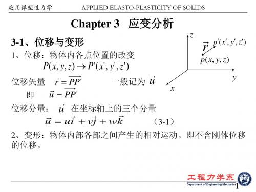
3-3、应变分量与位移分量之间的微分关系—几何方程:
应变是与位移有关的。物体中各质点相对位置的改变,则产生 变形。因此要分析物体的变形,就要研究各点的位置的变化。
v
xy
yx
v x
u y
x (3-5)
v(x, y) b
d
dy
yo
p
x
a
dx
p yx
a
v v(x dx, y)
u
dx u u
z u(x, y)
dx u
11
应用弹塑性力学
APPLIED ELASTO-PLASTICITY OF SOLIDS
x
y
z
v' v( x, y, z) v dx v dy v dz
x
y
z
w' w( x, y, z) w dx w dy w dz
x
y
z
14
应用弹塑性力学
APPLIED ELASTO-PLASTICITY OF SOLIDS
为了表示成应变分量的关系,对 u, v, w 作如下改写:
x
v v(x, y, z) v' v(x dx, y dy, z dz)
位移分量是坐标的函数 w w(x, y, z) w' w(x dx, y dy, z dz)
弹性力学2014_第三章
d 4 f y d 4 f1 y d 4 f2 y d 2 f y 0 0, 2 0 0, 0 4 4 4 2 dy dy dy dy f y Ay y 3 By y 2 Cy yD
2
§3-4 §3 4 简支梁受均布载荷
弹性力学与材料力学解答的比较 弹 学与 料 学解
y 2 3 M 6 q 2 y2 y 2 y3 x 3 yl qx 4 y 2q 4 2 I h h h5 h h 5 q y 2 y y 1 1 2 h h 2 FS6 S q h 2 y xy xy 3 x bI h 4
§3-1 逆解 § 逆解法与半逆解法 半逆解 多项式解 多项式解答
当体力为常量时,按应力求解平面问题,最后可以 归结为求解一个应力函数,它必须满足下列条件:
(1) 在区域内的相容方程
4 4 4 2 2 2 4 0 4 x x y y
4 0
(2) 在边界上的应力边界条件(假设全部为应力边界条件)
u M v M v u y, y, 0 x EI y EI x y
§3-3 §3 3 位移分量的求出
将前两式积分可以得到
M M 2 u xy y f1 y , v y f2 x EI EI v u 0 代入 代 x y df 2 x M df1 y df 2 x M df1 y x x 0 dx EI dy dx EI dy
应力的量纲 N/m2 以上分量的量纲 N/m3 因此应力的表达式可能为 A1 gx, B 1 gy, C 2 gx, D 2 gy 的组合
弹性力学双语讲义(Chapter4)
Only the circumferential displacement takes place只有环向位移
• the angle of rotation of PA will be =(AA-PP)/ PA =[(u+u/rdr)-u ]/dr= u/r • the angle of rotation of PB will be =<pop =- PP/OP=-u/r • rr =+=u/r-u/r
• the angle of rotation of PA will be =0 • the angle of rotation of PB will be =(BBPP)/PB=[(ur+ur/d)-ur]/rd=ur/(r) • rr =+=ur/(r)
9
13
rxy=u/y+v/x中的一般规律
• 由rxy=u/y+v/x,总结出一般规律,即设有 两个正交坐标方向,一个坐标方向的位移(如 u)对另一个坐标方向(y)求导为该坐标方向 (y)线段的转角。 1. u/y--x方向的位移 u 对y坐标求导为y方向线 段的转角。 2. v/x--y方向的位移 v 对x坐标求导为x方向线 段的转角。 • 应用这一规律于极坐标,就能方便地解释 ur/(r) +u/r为rr中的项。
4.2 geometrical and physical equations in polar coordinates极坐标中的几何物理方程
• P57(E) Fig. 4.2.1;P60(中)图4-2
7
Only the radial displacement takes place只有径向位移
12
x=u/x y=v/y中的规律
弹性力学第三章

u =u v=v
位移解法例题
单位厚度薄板,两侧均匀受压,上下刚性约束, 单位厚度薄板,两侧均匀受压,上下刚性约束,不计摩擦和 体力 位移场
u = u ( x) v=0
拉梅方程
E ′ ∂ 2u 1 −ν ' ∂ 2u 1 + ν ' ∂ 2 v ( 2+ + )=0 2 2 1 − ν ′ ∂x 2 ∂y 2 ∂x∂y E ′ ∂ 2 v 1 −ν ' ∂ 2 v 1 + ν ' ∂ 2u ( 2+ + )=0 2 2 1 − ν ′ ∂y 2 ∂x 2 ∂x∂y ∂ 2u =0 2 ∂x
第三章 平面问题的直角坐标解法 问题的简化
空间问题
特殊化
平面应力问题 平面问题 平面应变问题
问题的解法
位移解法 应力解法 应力函数解法
特殊问题的解
悬臂梁的弯曲解 均布横向荷载简支梁的弯曲解 任意横向荷载简支梁弯曲的三角级数解
平面应变问题
1)无限长的等直柱体; 2)在柱体侧面受到与轴线垂直,且沿轴向均布的面力 作用; 0 Tz = 3)体力也垂直于轴线,并沿轴线均布。Fz = 0
边界条件
力学边界条件
E′ ∂u 1 − ν ′ ∂u ∂v ' ∂v [ nx ( + ν ) + ny ( + )] = Tx 2 1 −ν ′ ∂x ∂y 2 ∂y ∂x E′ ∂v ∂u 1 − ν ′ ∂v ∂u ′ ) + nx [ny ( + ν ( + )] = Ty 2 1 −ν ′ ∂y ∂x 2 ∂x ∂y
− ∫ yσ x dy = M
h 下表面 y = + : 2 nx = 0, n y = 1
弹性力学第4章第3章PPT课件
9
D 由应力函数求解时所用公式 应力函数表示的相容方程为
4x 4 2x22y2 4y 4 0
x
2 y2
fxx
y
2 x2
fy
y
l x m yx fx
m y l xy f y
xy
2 xy
40
10
逆解法的主要步骤
• 就是先设定各种形式的、满足相容方程的应力函数;
40
• 再求出应力分量;
x
2 y2
fxx
y
2 x2
fy y
xy
2 xy
• 然后根据应力边界条件来考察, 在各种形状的弹性体上,
这些应力分量对应于什么样的面力, 从而得知所设定的应
2xy
xy
6
用应力表示的相容方程〈平面应力情况 )
x2 2 y2 2 xy 1 fx x fy y
用应力表示的相容方程(平面应变情况)
x22 y22 xy 1 1 fxx fyy
如体力与坐标无关(例如重力), 则
x22 y22x y 0
y
2 x 2
xy
2 xy
l x m yx fx
m y l xy f y
13
§3-1 多项式解答2
第三章 平面问题的直角坐标解答
用逆解法求出几个简单平面问题的多项式解答
假定体力可以不计 fx fy 0
取一次式 Φabxcy 相容方程总能满足!
x 0 y 0
xyyx0
fx fy 0
x
2 y 2
弹性力学简明教程第四版第三章课件

x2 f y xf1 y f 2 y 2
其中 f (y), f1(y), f2(y) 都是待定的 y 的函数。
3. 由相容方程求解应力函数
将 代入 得
4 4 4 2 2 2 0 4 4 y x y x
1 d 4 f y 2 d 4 f1 y d4 f2 y d2 f y x x 2 0 4 4 4 2 2 dy dy dy dy
1 d 4 f y 2 d 4 f1 y d4 f2 y d2 f y x x 2 0 4 4 4 2 2 dy dy dy dy
这是 x 的二次方程,但相容方程要求它有无数多的根 (全梁的 x 都应该满足它), 可见它的系数和自由项都 必须等于零,即 4 4 4 2
2 2 y 2 f y y, xy . x xy
4. 由应力函数求应力分量
将
2 代入 x y 2 f x x,
xy x3 Ay2 2 By C 3Ey2 2 Fy G
x2 x 6 Ay 2 B x6 Ey 2 F 2 Ay3 2 By2 Hy 2 K 2 y Ay3 By2 Cy D
q
于是,有
x
2
E=F=G=0
ql
xy x3 Ay2 2 By C
x 6 Ay 2B 2 Ay3 2By2 Hy 2K 2 y Ay3 By2 Cy D
O
l
h/2 h/2
ql x l
y
5. 考察边界条件(确定待定系数) 通常梁的跨度远大于梁的深度, 梁的上下两个边界是主要边界。 在主要边界上应力边界条件必须 完全满足;次要边界上如果边界 条件不能完全满足,可引用圣维 南原理用三个积分条件来代替。
- 1、下载文档前请自行甄别文档内容的完整性,平台不提供额外的编辑、内容补充、找答案等附加服务。
- 2、"仅部分预览"的文档,不可在线预览部分如存在完整性等问题,可反馈申请退款(可完整预览的文档不适用该条件!)。
- 3、如文档侵犯您的权益,请联系客服反馈,我们会尽快为您处理(人工客服工作时间:9:00-18:30)。
B.
=ax2 ,
X=0, Y=0
• 满足相容方程 4 =0 • 由下式求出应力分量 x=2/y2=0 y= 2/x2=2a xy=-2/xy=0 • 对和坐标轴平行的矩形板求出面力分量知 =ax2 能解决矩形板y向受均匀拉力(a>0)或 均 匀压力(a<0)的问题。P37 Fig.3.1.1(a)
13
E.
=ay3 ,
X=0, Y=0
• It satisfies the compatibility equation 满足相容方程 4 =0 • Find the stress components by 由下式求出应力分量 x=2/y2=6ay y= 2/x2=0 xy=-2/xy=0 • For a rectangular plate shown in fig.1, find the surface force components shown in fig.1对矩形 板求出面力分量,如图1所示。 • Solve the problem of pure bending of a rectangular beam. 矩形板纯弯曲问题
6
7
C.
=2 ,
X=0, Y=0
• It satisfies the compatibility equation 4 =0 • find the stress components by x=2/y2=2c y= 2/x2=0 xy=-2/xy=0 for a rectangular plate with its edges parallel to the coordinate axes, find the surface force components by (lx+m yx)s=X (my+lxy)s =Y • the stress function =cy2 can solve the problem of uniform tension (c>0) or uniform compression (c<0) of a rectangular plate in x direction. P37 Fig.3.1.1(c)
17
Integration of geometrical equations x=u/x y=v/y rxy=u/y+v/x 几何方程的积分 • substitution of strains into the geometrical equations (2.4.6) yields 将应变代入几何方程 u/x =My/(EI) u=Mxy/(EI)+f(y) v/y = -My/(EI) v= -My2/(2EI)+g(x) u/y+v/x=0 -df(y)/dy=dg(x)/dx+Mx/(EI)
8
C.
=cy2 ,
X=0, Y=0
• 满足相容方程 4 =0 • 由下式求出应力分量 x=2/y2= 2c y= 2/x2=0 xy=-2/xy=0 • 对和坐标轴平行的矩形板求出面力分量知 =cy2 能解决矩形板x向受均匀拉力(c>0)或 均 匀压力(c<0)的问题。P37 Fig.3.1.1(c)
14
15
E.
• Fig 1
=ay3 ,
X=0, Y=0
• Fig 2 • statically equivalent systems 静力等效 a=2M/h3 • x=6ay=12My/h3=My/I I=h3/12 y= 0 xy=0
16
3.2 Determination of displacements when x=My/I y= 0 xy=0 位移的确定 • In the case of plane stress, substitution of stresses into the physical equations(2.6.4) yields 平面应力问题,将应力代入物理方程得 应变 x=[x- y]/E =My/(EI) y=[y- x]/E = - My/(EI) rxy=xy/G =0
4
B.
=ax2 ,
X=0, Y=0
• It satisfies the compatibility equation 4 =0 • find the stress components by x=2/y2=0 y= 2/x2=2a xy=-2/xy=0 • for a rectangular plate with its edges parallel to the coordinate axes, find the surface force components by (lx+m yx)s=X (my+lxy)s =Y • the stress function =ax2 can solve the problem of uniform tension (a>0) or uniform compression (a<0) of a rectangular plate in y direction. P37 Fig.3.1.1(a)
18
Separation of variables 分离变量 -df(y)/dy=dg(x)/dx+Mx/(EI)= • -df(y)/dy= f(y)=- y+u0 • dg(x)/dx+Mx/(EI)= g(x)= - Mx2/(2EI)+x+v0 • u=Mxy/(EI)- y+u0 (3.2.5) v= -My2/(2EI)-Mx2/(2EI)+x+v0 (3.2.6) =u/y= Mx/(EI)- ----the cross section remains plane after bending 横截面弯曲变形后仍 为平面。 1/ = 2v/x2 =- M/(EI) ----all the longitudinal lines will have the same curvature曲率相同
2
A.
=a+bx+cy ,
X=0, Y=0
• It satisfies the compatibility equation 4 =0 • find the stress components by x=2/y2=0 y= 2/x2=0 xy=-2/xy=0 • find the surface force components by (lx+m yx)s=X=0 (my+lxy)s =Y=0 • a linear stress function corresponds to the case of no surface forces and no stress . • The superposition of a linear function to the stress function for any problem does not affect the stresses.
3
A.
=a+bx+cy ,
X=0 Y=0
• 满足相容方程 4 =0 • 由下式求出应力分量 x=2/y2=0 y= 2/x2=0 xy=-2/xy=0 • 由下式对给定坐标的物体求出面力分量 (lx+m yx)s=X=0 (my+lxy)s =Y=0 • 确定所设定的 能解决的问题为:任意物体无 体力,无面力,无应力。 • 应力函数加或减一个线性项不影响应力。
19
Review: Rigid-body displacements-displacements corresponding to zero strains 刚体位移--应变为零时的位移 • u= - y +u0 v= x+v0
• u0--the rigid-body translation in the x direction x向刚体平动 • v0--the rigid-body translation in the y direction y向刚体平动
9
10
D.
=bxy ,
X=0, Y=0
• It satisfies the compatibility equation 4 =0 • find the stress components by x=2/y2=0 y= 2/x2=0 xy=-2/xy=-b • for a rectangular plate with its edges parallel to the coordinate axes, find the surface force components by (lx+m yx)s=X (my+lxy)s =Y • the stress function =bxy can solve the problem of a rectangular plate in pure shear. P37 Fig.3.1.1(b)
22
3.3 Bending of a simple beam under uniform load简支梁在均布荷载作用下的弯曲
• A simple beam ,length 2L, depth h, uniform load q. P41 fig.3.3.1
23
Semi-inverse method: 半逆解法 assume 假定y= 2/x2=f(y)
• Successive integration with respect to x yields 对x连续积分二次得 /x=xf(y) +f1(y) =x2 f(y)/2 +xf1(y)+f2(y) • substitution of into compatibility equation (4/x4+24/x2y2 +4/y4)=0 (2.12.11) yields 将代入相容方程得: x2/2 f(4)(y)+xf1(4)(y)+f2(4)(y)+2f”(y)=0