Chapter 3The Consumer’s Problem(高级微观经济学-上海财经大学,沈凌)
范里安《微观经济学(高级教程)》(第3版)章节题库-不确定性(圣才出品)
第11章不确定性一、判断题1.对于两种赌博,不论他们的期望报酬怎样,一个风险厌恶者总会选择方差小的那种。
()【答案】F【解析】风险厌恶者更加偏好的是财富的期望值,而不是赌博本身。
因此,期望报酬对风险厌恶者的选择是有影响的。
当期望报酬相等,风险厌恶者总会选择方差小的那种。
2.某消费者不属于风险厌恶者。
他有机会通过支付10元去买一张彩票,这张彩票将使他以0.05的概率赢得100元,以0.1的概率赢得50元,有0.85的概率他将一无所获。
如果他明白胜算的可能并且计算没有错误,那么他将买下彩票。
()【答案】T【解析】买彩票的期望效用为:()()()⨯+⨯+⨯。
买彩票和不买彩0.051000.1500.850u u u票的期望收益是相等的,对于一个非风险厌恶者来说,有:()()()()()u u u u u⨯+⨯+⨯≥⨯+⨯+⨯=0.051000.1500.8500.051000.1500.85010因此他将买下彩票。
3.如果保险费用上升,人们将减少风险厌恶程度。
()【答案】F【解析】并不是由保险费用来决定风险厌恶程度,而是由风险厌恶程度来决定保险费用。
对于风险厌恶者来说,完全保险是他的最优选择;而风险偏好者对保险的需求并没有前者大。
4.某消费者有冯·诺依曼-摩根斯顿效用函数()()(),,,a b a b a a b b u c c p p p v c p v c =+。
a p 和b p 分别是事件a 和事件b 发生的概率,a c 和b c 分别是以事件a 和事件b 而定的消费。
如果()v c 是一个增函数,这个消费者必定是风险爱好者。
()【答案】F【解析】()v c 是一个增函数,则()0v'c >。
()()()0a b a b a a b b u'c c p p p v'c p v'c =+>,,,,()()(),,,a b a b a a b b u''c c p p p v''c p v''c =+。
《高级宏观经济学》教学大纲(硕士研究生)-RonaldoCarpio

《高级宏观经济学》教学大纲(硕士研究生) - RonaldoCarpio《高级微观经济分析》教学大纲(博士研究生)课程代码:(按本专业或方向培养方案填写)课程名称:(按本专业或方向培养方案填写)英文名称:Advanced Microeconomic Analysis课程性质:(按本专业或方向培养方案填写)学分学时:3学分,48学时授课对象:金融学院一年级博士研究生课程简介:Based on Microeconomics I (for master students), the course will discuss thecontemporary development in microeconomics. This course is also designed to develop andextend the students’ analytical and reading skills in modern microeconomics. A student who haspassed the course should be able to read typical articles in the mainline journals, understand theanalytical derivations and arguments commonly used in the literature, and know how to solve themore widely used models.先修课程:Microeconomics for master students选用教材:1、 Mas-Colell, A., M. D. Whinston, and J. Green, Microeconomic Theory. (MWG)2、 Jehle, Geoffrey A. and Philip J. Reny, Advanced Microeconomic Theory. (JR)考核方式与成绩评定:Final Exam %; Midterm Exam %; Class Participation % 主讲教师:Carpio Ronaldo、颜建晔所属院系:金融学院联系方式:******************、*******************答疑时间及地点:求索楼123,Wednesday 13:30-14:30 (Carpio),Tuesday 15:00-17:00(颜)第一章:Consumer Theory教学目标和要求:Understand the consumer’s problem and consumer demand.教学时数:6学时教学方式:讲授准备知识:calculus教学内容:Preferences, Utility, and Consumer’s Problem第一节:Consumer’s Problem第二节:Indirect Utility, Demand作业与思考题:JR Ch 1.6参考资料:JR Ch 1, Appendix A1, A21第二章: Topics in Consumer Theory教学目标和要求:Understand duality, integrability, and uncertainty.教学时数:6 学时教学方式:讲授准备知识:statistics教学内容:Duality, Integrability, and Uncertainty 第一节:Duality of Consumer’s Problem第二节:Revealed Preferences & Uncertainty 作业与思考题:JR Ch 2.5 参考资料:JR Ch 2第三章: Theory of the Firm教学目标和要求:Understand the firm’s profit maximization problem.教学时数:6 学时教学方式:讲授准备知识:Chapter 1,2教学内容:Production, Cost, Profit Maximization 第一节:Production Functions & Cost第二节:Duality in Production, Competitive Firms 作业与思考题:JR Ch 3.6参考资料:JR Ch 3第四章: Partial Equilibrium教学目标和要求:Understand partial equilibrium markets. 教学时数:3学时教学方式:讲授准备知识:Chapter 3教学内容:Perfect & Imperfect Competition, Welfare 第一节:Competition 第二节:Equilibrium & Welfare作业与思考题:JR Ch 4.4参考资料:JR Ch 4第五章: Walras’/competitive equilibrium2教学目标和要求:competitive market economies from a Walrasian (general) equilibrium perspective.Let students understand “why the competitive market/equilibrium may work or fail?”教学时数:6学时方式:讲授教学准备知识:consumer theory, production theory教学内容:第一节:Walrasian economy and mathematical language of microeconomics 第二节:competitive equilibria of pure exchange and with production 作业与思考题:JR5.5, exercises of MWG Ch15, 18, 教师自编习题集参考资料:MWG Mathematical Appendix, Ch15, 18; JR5.4第六章: Social choice function/theory and social welfare: normative aspect of microeconomics教学目标和要求:When we judge some situation, such as a market equilibrium, as “good”or “bad”, or “better” or “worse” than another, we necessarily make at least implicit appeal to some underlying ethical standard. Welfare economics helps to inform the debate on social issues by forcingus to confront the ethical premises underlying our arguments as well as helping us to seetheir logical implications.Let students have a systematic framework for thinking about normative and social welfare topics.教学时数:3学时教学方式:讲授准备知识:Walrasian equilibrium教学内容:第一节:social choice, comparability, and some possibilities第二节:Rawlsian, Utiliterian, and flexible forms作业与思考题:JR6.5, exercises of MWG Ch21, 22, 教师自编习题集参考资料:MWG Ch21.A, Ch21.E, Ch22.C; JR Ch6第七章: Strategic Behavior and Asymmetric Information教学目标和要求:A central feature of contemporary microeconomicsafter Walrasian economy is the multi-agent interaction which represents the potential for the presence of strategicinterdependence. Let students grasp classic models of imperfect competition under symmetric and asymmetric information.3教学时数:3学时教学方式:讲授准备知识:perfect competition教学内容:第一节:monopoly and oligopoly under symmetric information第二节:oligopoly under asymmetric information作业与思考题:教师自编习题集参考资料:MWG Ch12; JR Ch4第八章: Theory of Incentives教学目标和要求:The strategic opportunities that arise in the presence of asymmetricinformation typically lead to inefficient market outcomes, a form of market failure. Underasymmetric information, the first welfare theorem no longer holds generally. Thus, the main themeto be explored is to stimulate different agents’ optimal/efficient behaviors in differentinformational settings to achieve the “second-best” market outcomes.教学时数:9学时教学方式:讲授准备知识:Strategic Behavior and Asymmetric Information教学内容:第一节:Adverse selection第二节:Moral hazard*第三节:Task separation/integration,第三节:Career concern作业与思考题:exercises of MWG Ch13, 14, 教师自编习题集参考资料:JR Ch8; MWG Ch13, 14第九章前沿研究讲座:待定邀请校外老师(待定)给学生们讲演最新研究,引导学生讨论;在学生掌握现代微观经济学基本模型之后能够接触到前沿研究。
微观经济学:现代观点(范里安-著)48题及答案汇编

第一部分 消费者选择理论1.有两种商品,x1和x2,价格分别为p1和p2,收入为m 。
当11x x ≥时,政府加数量税t,画出预算集并写出预算线2. 消费者消费两种商品(x1,x2),如果花同样多的钱可以买(4,6)或(12,2),写出预算线的表达式。
3.重新描述中国粮价改革(1)假设没有任何市场干预,中国的粮价为每斤0。
4元,每人收入为100元。
把粮食消费量计为x ,在其它商品上的开支为y ,写出预算线,并画图。
(2)假设每人得到30斤粮票,可以凭票以0。
2元的价格买粮食,再写预算约束,画图。
(3)假设取消粮票,补贴每人6元钱,写预算约束并画图。
4. 证两条无差异曲线不能相交5. 一元纸币(x1)和五元纸币(x2)的边际替代率是多少? 6. 若商品1为中性商品,则它对商品2的边际替代率?7. 写出下列情形的效用函数,画出无差异曲线,并在给定价格(p 1,p 2)和收入(m )的情形下求最优解。
(1)x 1=一元纸币,x 2=五元纸币。
(2)x 1=一杯咖啡,x 2=一勺糖, 消费者喜欢在每杯咖啡加两勺糖。
8. 解最优选择 (1)21212(,)u x x x x =⋅(2)2u x =+9. 对下列效用函数推导对商品1的需求函数,反需求函数,恩格尔曲线;在图上大致画出价格提供曲线,收入提供曲线;说明商品一是否正常品、劣质品、一般商品、吉芬商品,商品二与商品一是替代还是互补关系。
(1)212x x u += (2)()212,m in x x u =(3)ba x x u 21⋅=(4) 12ln u x x =+,10. 当偏好为完全替代时,计算当价格变化时的收入效用和替代效用(注意分情况讨论)。
11. 给定效用函数 (,)x y xy =,p x =3,p y =4,m=60,求当p y 降为3时价格变化引起的替代效应和收入效应。
12. 用显示偏好的弱公理说明为什么Slutsky 替代效应为负。
高级微观经济学-教学大纲

⾼级微观经济学-教学⼤纲《⾼级微观经济学》教学⼤纲“Advanced Microeconomics” Course Outline课程编号:151193A课程类型:专业选修课总学时:48 讲课学时:48学分:3适⽤对象:经济学、统计学、⾦融学先修课程:经济学原理、中级微观经济学、线性代数、微积分Course Code: 151193ACourse Type: Specialized elective coursePeriods: 48 Lecture: 48Credits: 3Applicable Subjects: Economics, Statistics, FinancePreparatory Courses: Principles of Microeconomics, Introductory Microeconomics, Linear Algebra, Mathematical Analysis⼀、课程的教学⽬标本课程作为本科学⽣的专业选修课旨在通过介绍微观经济学中的主要模型、原理和证明使学⽣具备进⾏微观经济学研究的基本⽅法与技能,为后续专业课程的学习奠定基础。
This specialized elective course is offered to undergraduate students majoring in Economics, Statistics, and Finance. This course builds the foundation for the study of subsequent major courses and trains the students in the micro – economic research skills.⼆、教学基本要求本课程的教学内容⼤致可以分为四⼤部分。
第⼀部分为个⼈决策理论。
第⼆部分为博弈论。
第三部分为市场均衡和市场失效理论。
高级微观经济学讲义 (1)
5.Relationship
• Hicks demand and expenditure function:
h(p, u ) p e(p, u )
2 – D p h(p, u ) D p e(p, u ) is s.n.s.d.
• Hicks and Walras demand:
3.Utility maximization
• Consumer’s problem (UMP):
max u ( x)
x0
s.t.
x B(p.w)
• The solutions x(p.w) are called Walras’ Demand Correspondence, or function if it’s single point.
3.Utility maximization
• Properties of x(p.w)
– HD0 – Satisfied Walras’ Law – If % are concave, x(p.w) are concave too, if % are strictly concave, x(p.w) is single point.
– % is local non-satiation: x X, and >0 there is a y, that y-x ,and y x
• proposition3: % is strong monotone, then it’s monotone; % is monotone, it’s local non-satiation.
2.From preferences to utility
• Convexity: x upper contour sets are convex.
范里安《微观经济学(高级教程)》(第3版)课后习题-均衡分析(圣才出品)
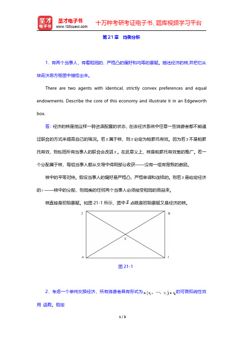
第21章均衡分析1.有两个当事人,有着相同的、严格凸的偏好和均等的禀赋。
描述经济的核,并把它从埃奇沃思方框图中描绘出来。
There are two agents with identical,strictly convex preferences and equal endowments.Describe the core of this economy and illustrate it in an Edgeworth box.答:经济的核是指这样一种资源配置的状态,在该经济系统中任意一些消费者都不能通过联合的方式来提高自己的境况。
若x属于核,则x必定为帕累托有效。
因为若x不是帕累托有效,则包括所有当事人的联合会改进x。
在此意义上,核是帕累托有效集的推广。
若一个分配属于核,每组当事人都从交易中得到部分收获——没有一组有背叛的激励。
核中的平等对待。
假设当事人的偏好是严格凸,严格单调和连续的。
则若x是给定经济的r——核中的分配,则同类的任何两个当事人必须接受相同的商品束。
核直接是初始禀赋。
如图21-1所示,图中E点既是初始禀赋又是经济的核。
图21-12.考虑一个单纯交换经济,所有消费者具有形式为的可微拟线性效用函数。
假定是严格凹的。
证明均衡唯一。
Consider a pure exchange economy in which all consumers have differentiable quasilinear utility functions of the form ()10n u x x x +,…,.Assume that ()1n u x x ,…,is strictly concave.Show that equilibrium must be unique.证明:均衡的唯一性。
假设z 是一个定义于价格单形上的具有连续导函数的总超额需求函数,且当0i p =时,有()0i z p >。
英文版微观经济学复习提纲Chapter 3.the interaction of demand and supply
3Where Prices Come From: The Interaction of Demandand SupplyChapter SummaryThe model of demand and supply explains how prices are determined in a market system. The main factor affecting the demand for a product is its price. A demand schedule lists various prices of a product and the quantities demanded at those prices. A demand curve shows this same relationship in a graph. The law of demand is the negative relationship between price and quantity demanded, holding everything else constant. Other factors that affect demand include prices of related goods (substitutes and complements), income, tastes, population and demographics, and expected future prices. Responses to changes in any of these shift a product’s demand curve and are called changes in demand.The most important factor affecting the supply of a product is its price. A supply schedule lists various prices of a product and the quantities supplied at those prices. A supply curve shows this same relationship in a graph. The law of supply is the positive relationship between price and quantity supplied, holding everything else constant. Other factors that affect supply include prices of inputs, technological change, prices of substitutes in production, expected future prices, and the number of firms in the market. In response to a change in any one of these factors there will be a change in supply or a shift in the supply curve.The intersection of demand and supply creates an equilibrium price. A surplus exists when the price charged is above the equilibrium price. A shortage exists when the price charged is below the equilibrium price. When the price charged equals the equilibrium price both consumers and producers are willing to exchange the same quantity of the product and there is no further movement in the market price.An increase in demand increases equilibrium price and increases the equilibrium quantity. A decrease in demand decreases equilibrium price and decreases the equilibrium quantity. An increase in supply decreases equilibrium price and increases the equilibrium quantity. A decrease in supply increases equilibrium price and decreases the equilibrium quantity.Learning ObjectivesWhen you finish this chapter you should be able to:1.Understand the factors that influence the demand for goods and services. Many factorsinfluence the willingness of consumers to buy a particular product. Among these factors are theincome they have to spend and the effectiveness of advertising campaigns of the companies that sellproducts consumers want. The most important factor in consumer decisions, though, is the price ofthe product. It is important to note that demand refers not to what a consumer wants to buy but whatWhere Prices Come From: The Interaction of Demand and Supply 33 the consumer is both willing and able to buy. In other words it’s not only what consumers want butalso what they can afford.2.Understand the factors that influence the supply of goods and services. Just as many variablesinfluence consumer demand, many variables influence the willingness and ability of firms to sell agood or service. Among these variables are the prices of inputs used in production and the number offirms in the market. The most important variable that affects firms is the price of whatever they sell.3.Explain how equilibrium in a market is reached, and use a graph to illustrate marketequilibrium. Economists use graphs to show how demand and supply interact in a competitivemarket to establish equilibrium. The graph of a competitive market shows that quantity demandedequals quantity supplied at the equilibrium price. When the price is greater than the equilibriumprice, a surplus exists. In response to the surplus the market price will fall to the equilibrium level.When the price is less than the equilibrium price, a shortage exists. In response to the shortage themarket price will rise to the equilibrium level.e demand and supply graphs to predict changes in prices and quantities. Demand and supplyin most markets change constantly. As a result, equilibrium prices and quantities change constantly.Graphs show the impact on competitive market equilibrium of increases and decreases in demandand supply.Chapter ReviewChapter Opener: How Hewlett-Packard Manages the Demand for PrintersHewlett-Packard (H-P) is a leading selling of printers in the United States. The firm’s success depends on the ability of its executives to analyse and react to changes in the demand and supply of its products. HP’s ability to sell printers is closely tied to the sales of computers and digital cameras. The strength of the overall economy also affects H-P’s business. For example, when the U.S. economy experienced a recession in 2000, sales of computers and printers fell.Helpful Study HintHewlett-Packard and the market for printers are used throughout the chapter to demonstrate changes in demand and supply and how they affect prices. At the end of this chapter An Inside Look describes the competition the company faces in the markets for personal computers and printers.The Demand Side of the MarketAlthough many factors influence the willingness of consumers to buy a particular product the main influence on consumer decisions is the product’s price. The quantity demanded of a good or service is the amount that a consumer is willing and able to purchase at a given price. A demand schedule is a table showing the relationship between the price of a product and the quantity of the product demanded. A demand curve shows this same relationship in a graph. Because quantity demanded always increases in response to a decrease in34 Chapter 3price, this relationship is called the law of demand. The law of demand is explained by the substitution and income effects. The substitution effect is the change in quantity demanded of a good that results from a change in price, making the good more or less expensive relative to other goods that are substitutes for it. The income effect is the change in the quantity demanded of a good that results from the effect of a change in the good’s price on consumer purchasing power.Ceteris paribus (“all else equal”) is the requirement that when analysing the relationship between two variables - such as price and quantity demanded - other variables must be held constant. When one of the non-price factors that influence demand changes a shift in demand - an increase or decrease in demand - results. The most important non-price influences on demand are prices of related goods (substitutes and complements), income, tastes, population and demographics and expected future prices.Substitutes are goods and services that can be used for the same purpose while complements are goods that are used together. A decrease in the price of a substitute for good A causes the quantity of the substitute demanded to increase, shifting the demand curve for good A to the left. An increase in the price of a substitute for good A causes the quantity of the substitute demanded to decrease, shifting the demand curves for good A to the right. Changes in prices of complements have the opposite effect. A decrease in the price of a complement for good B causes the quantity of the complement demanded to increase, shifting the demand curve for good A to the right. An increase in the price of a complement for good B causes the quantity of the complement demanded to decrease, shifting the demand curve for good A to the left.The income that consumers have available to spend affects their willingness to buy a good. A normal good is a good for which demand increases as income rises and decreases as income falls. An inferior good is a good for which demand increases as income falls and decreases as income rises. When consumers’ tastes for a product increase, the demand curve for the product will shift to the right, and when consumers’ tastes for a product decrease, the demand curve for the product will shift to the left.As population increases, the demand for most products increases. Demographics are the characteristics of a population with respect to age, race, and gender. As demographics change the demand for particular goods will increase or decrease because different categories of people will have different preferences for those goods. If enough consumers become convinced that a good will be selling for a lower price in the near future, the demand for the good will decrease in the present. If enough consumers become convinced that the price of a good will be higher in the near future, the demand for the good will increase in the present.Helpful Study HintStudents often confuse a change in quantity demanded with a change in demand. Only one variable, the price of a good or service, can cause changes in quantity demanded. This change is described as a movement along a demand curve. Changes in demand are caused by changes in non-price factors. Constant repetition is essential to understand this important difference. Use Making the Connection 3.1 (page 68) and Making the Connection 3.2 (page 81) to find examples of factors that change demand. Be sure you understand why it is demand and not quantity demanded that changes.The Supply Side of the MarketMany variables influence the willingness of firms to sell a good or service. The most important of these variables is price. Quantity supplied is the amount of a good or service that a firm is willing to sell at a givenWhere Prices Come From: The Interaction of Demand and Supply 35 price. A supply schedule is a table that shows the relationship between the price of a product and the quantity of the product supplied. A supply curve shows this same relationship in a graph. The law of supply states that, holding everything else constant, increases in price cause increases in the quantity supplied and decreases in price cause decreases in the quantity supplied.Variables other than price affect supply. When any of these variables change, a shift in supply - an increase or a decrease in supply - results. The following are the most important variables that shift supply: prices of inputs used in production, technological change, prices of substitutes in production, expected future prices and the number of firms in the market.If the price of an input (for example, labour or energy) used to produce a good rises, the supply for the good will decrease and the supply curve will shift to the left. If the price of an input decreases, the supply for the good will increase and the supply curve will shift to the right. Technological change is a positive or negative change in the ability of a firm to produce a given level of output with a given amount of inputs. A positive technological change will shift a firm’s supply curve to the right while a negative technological change will shift a firm’s supply curve to the left.An increase in the price of an alternative good (B) that a firm could produce instead of producing good A will shift the firm’s supply curve for good A to the left. If a firm expects the price of its product will rise in the future, the firm has an incentive to decrease supply in the present and increase supply in the future. When firms enter a market, the market supply curve shifts to the right. When firms exit a market, the market supply curve shifts to the left.Helpful Study HintThe law of supply may seem logical because producers earn more profit when the price they sell their products for rises. But consider Figure 3.7 (pages 72-73) and the following question: “If Hewlett-Packard can earn a profit from selling 9 million printers per month at a price of $125, why not increase quantity supplied to 10 million and make even more profit?” The upward slope of the supply curve is due not only to the profit motive but the increasing marginal cost of printers. (Increasing marginal costs were discussed in Chapter 2.) Hewlett-Packard will increase its quantity supplied from 9 to 10 million in Figure 3.7 only if the price it will receives is $175 because the cost of producing one million more printers is greater than the cost of the last one million printers.As with demand and quantity demanded, be careful not to confuse a change in quantity supplied (due only to a change in the price of a product) and a change in supply (a shift of the supply curve in response to one of the non-price factors). Constant reinforcement of this is necessary. Be careful not to refer to an increase in supply as “a downward shift” or a decrease in supply as “an upward shift.” Because demand curves are downward-sloping, an increase in demand appears in a graph as an “upward shift.” But because supply curves are upward-sloping, a decrease in supply appears in a graph as an “upward shift.” You should always refer to both changes in demand and supply as being “shifts to the right” and “shifts to the left” to avoid confusion.36 Chapter 3Market Equilibrium: Putting Demand and Supply TogetherThe purpose of markets is to bring buyers and sellers together. The interaction of buyers and sellers in markets results in firms producing goods and services consumers both want and can afford. At market equilibrium the price of the product makes quantity demanded equal quantity supplied. A competitive market equilibrium is a market equilibrium with many buyers and many sellers. The market price (the actual price you would pay for the product) will not always be the equilibrium price. A surplus is a situation in which the quantity supplied is greater than the quantity demanded. When there is surplus the market price is above the equilibrium price. Firms have an incentive to increase sales by lowering price. As the market price is lowered, quantity demanded will rise and quantity supplied will fall until the market reaches equilibrium.A shortage is a situation in which quantity demanded is greater than the quantity supplied. When there is a shortage the market price is below the equilibrium price. Some consumers will want to buy the product at a higher price to make sure they get what they want. As the market price rises the quantity demanded will fall - not everyone will want to buy at a higher price - and quantity supplied will rise until the market reaches equilibrium. At the competitive market equilibrium there is no reason for the price to change unless either the demand curve or the supply curve shifts.Helpful Study HintIt’s very important to understand how demand and supply interact to reach equilibrium. Remember that adjustments to a shortage and a surplus reflect changes in quantity demanded (not demand) and quantity supplied (not supply). Solved Problem 3.1 (page 80-81) addresses this. Market or actual prices are easy to understand because these are the prices consumers are charged. You know the price you paid for a CD because it is printed on the receipt. But no receipt has “equilibrium price” written on it.To help you understand what an equilibrium price and quantity are, it may help to use an analogy. Suppose you were to push an inflated ball under the surface of a sink filled with water. If you were to release the ball it would move quickly to the surface. If you were to hold the ball above the sink and drop it, the ball would fall to the surface. The surface of the water is the equilibrium position for the ball. A market equilibrium is the position a market will move towards if there is a shortage or surplus.The Effect of Demand and Supply Shifts on EquilibriumWhen the supply curve shifts, the equilibrium price and quantity change in the opposite direction. Increases in supply result from the following non-price factor changes: a decrease in an input price, positive technological change, a decrease in the price of a substitute in production, a lower expected future product price and an increase in the number of firms in the market. A decrease in supply results in a higher equilibrium price and a lower equilibrium quantity. Decreases in supply result from the following non-price factor changes: an increase in an input price, negative technological change, an increase in the price of a substitute in production, a higher expected future product price and a decrease in the number of firms in the market.When the demand curve shifts, the equilibrium price and quantity shift in the same direction. Increases in demand can be caused by any change in a variable that affects demand except price. For example, demand willWhere Prices Come From: The Interaction of Demand and Supply 37 increase if the price of a substitute rises, the price of a complement falls, income rises (for a normal good), income falls (for an inferior good), population increases or the expected future price of the product rises. A decrease in demand results in a lower equilibrium price and lower equilibrium quantity. Decreases in demand can be caused by any change in a variable that affects demand except price. For example, demand will decrease if the price of a substitute falls, the price of a complement rises, income falls (for a normal good), incomes rises (for an inferior good), population decreases, or the expected future price of the product falls.Helpful Study HintMaking the Connection 3.2 (page 81), Solved Problem 3.2 (pages 83-85) and questions 11-14 of the Problems and Applications can be used to conduct your own research on how changes in supply and demand affect prices in your community for products such as flat-screen televisions, watermelons and housing. For example, visit stores that sell flat-screen televisions and find out their market prices. Compare the market price you find with the expected prices as described in Making the Connection 3.2. For watermelons ask sellers how current prices compare with prices at different times of the year. Draw demand and supply diagrams that represent the market conditions you observe. You can ask your instructor if your analysis is correct.Solved ProblemChapter 3 of the textbook includes two Solved Problems that support learning objectives 1 (“Use a graph to illustrate market equilibrium”) and 4 (“Use demand and supply graphs to predict changes in prices and quantities”). The following is an additional Solved Problem that supports another learning objective from this chapter.Solved Problem 3.3 Supports Learning Objective 3.2: Understand the factors that influence the supply of goods and services.‘A farmer went to market to market to sell a…’Television programming in many parts of regional Australia features many commercials aimed at farmers. Ads for fertiliser, seed, and farm equipment are as common as commercials for laundry soap and soft drinks. Much of the nation’s wheat is grown in areas where the climate and soil conditions are well-suited for growing barley as well. Each year a farmer must decide how many acres of land to plant with wheat and how many acres to plant with barley.a)If both crops can be grown on the same land, why would a farmer choose to produce wheat ratherthan barley?b)Which of the variables that influence supply would explain a farmer’s choice to produce barley orwheat?Solving the ProblemStep 1: Review the chapter material. This problem refers to factors variables that affect supply, so you may want to review the section “Variables That Shift Supply,” which begins on pages 72-75 of the textbook.38 Chapter 3Step 2: Answer question (a) by explaining why a farmer would choose to produce wheat rather than barley. Among the factors that would influence a farmer’s choice is the expected profitability of the two crops.A farmer will grow wheat rather than barley if he expects the profits from growing wheat will be greater than those earned from growing barley.Step 3: Answer question (b) by explaining which variables may affect the farmer’s choice. Other things being equal, as the price of barley falls relative to the price of wheat, the supply of wheat would rise. Because wheat and barley are substitutes in production the variable “prices of substitutes in production” is the variable that would explain the farmer’s choice.Self-Test(Answers are provided at the end of the Self-Test.)Multiple-Choice Questions1.What does the term quantity demanded refer to?a.The total amount of a good that a consumer is willing to spend per month.b.The quantity of a good or service demanded that corresponds to the quantity supplied.c.The quantity of a good or service that a consumer is willing to purchase at a given price.d.None of the above2.Which of the following is the textbook’s definition of demand curve?a.The quantity of a good or service that a consumer is willing to purchase at a given price.b. A table showing the relationship between the price of a product and the quantity of theproduct demanded.c. A curve that shows the relationship between the price of a product and the quantity of theproduct demanded.d.The demand for a product by all the consumers in a given geographical area.Where Prices Come From: The Interaction of Demand and Supply 39 3.Refer to the graph below. What happens to quantity demanded in this graph?a.It increases as the price increases.b.It increases as the price decreases.c.It may increase or decrease as the price increases.d.It is not related to price.4.When the price of a printer rises, the quantity of printers demanded by Kate falls. According to thisstatement, what do we call Kate’s demand curve for printers?a.Unpredictableb.Upward slopingc.Downward slopingb.An exception to the law of demand5.If there are three consumers in a market, how can market demand be obtained?a.By adding the prices that consumers are willing to pay for a given quantity of output.b. b.By adding the quantities that consumers are willing to purchase at a given price, forvarious price levels.c.By adding both the prices consumers are willing to pay and the quantities consumers arewilling to purchase.d.By dividing the quantity demanded in the market by three.40 Chapter 36.What is the law of demand?a.The law of demand states that a change in the quantity demanded, caused by changes inprice, makes the good more or less expensive relative to other goods.b.The law of demand states that a change in the quantity demanded, caused by changes inprice, affects a consumer’s purchasing power.c.The law of demand states that, holding everything else constant, when the price of goodfalls, the quantity demanded will increase.d.The law of demand is the requirement that when analysing the relationship between priceand quantity demanded, other variables must be held constant.7.Which of the following best describes how consumers consider buying other goods when the price ofa good rises?a.The law of demandb.The substitution effectc.The income effectb.The term ceteris paribus8.Refer to the graphs below. Each graph refers to the demand for printers. Which of the graphs bestd escribes the impact of an increase in the price of a substitute good?a.The graph on the leftb.The graph on the rightc.Both graphsd.Neither graphWhere Prices Come From: The Interaction of Demand and Supply 41 9.Refer to the graphs below. Each graph refers to the demand for printers. Which of the graphs bestdescribes the impact of an increase in income, assuming that printers are a normal good?a.The graph on the leftb.The graph on the rightc.Both graphsb.Neither graph10.Refer to the graphs below. Each graph refers to the demand for printers. Which of the graphs bestdescribes the impact of an increase in population?a.The graph on the leftb.The graph on the rightc.Both graphsd.Neither graph11.When two goods are complements, which of the following occurs?a.The two goods can be used for the same purpose.b.The two goods are used together.c.The demand for each of these goods increases when income rises.d.The demand for each of these goods increases as income falls.12.What is an inferior good?a. A good for which demand increases as income risesb. A good for which demand decreases as income risesc. A good that cannot be used together with another goodb. A good that does not serve any real purpose13.Refer to the graph below. Which of the following moves best describes a change in demand?a.The move from A to Bb.The move from A to Cc.Either the move from A to B or the move from A to Cd.The move from B to A14.Refer to the graph below. Which of the following moves best describes what happens when a changein something other than the price of printers affects the market demand for printers?a.The move from A to Bb.The move from A to Cc.Either the move from A to B or the move from A to Cb.None of the above15.What does the term quantity supplied refer to?a.The quantity of a good or service that a firm is willing to supply at a given priceb. A table that shows the relationship between the price of a product and the quantity of theproduct suppliedc. A curve that shows the relationship between the price of a product and the quantity of theproduct demandedd.None of the above16.Which of the following is the textbook’s definition of supply curve?a.The quantity of a good or service that a firm is willing to supply at a given priceb. A table that shows the relationship between the price of a product and the quantity of theproduct suppliedc. A curve that shows the relationship between the price of a product and the quantity of theproduct suppliedd.None of the above17.Which of the following statements is correct?a.Once we know the market supply curve, we also know all the individual supply demandcurves.b.To derive a market supply curve, we add the prices that producers must obtain in order toproduce a given quantity of output.c.To derive a market supply curve, we can add horizontally individual supply curves.d.All of the above statements are correct.18.Refer to the graphs below. Each graph refers to the supply for printers. Which of the graphs bestdescribes the impact of an increase in the price of an input?a.The graph on the leftb.The graph on the rightc.Both graphsd.Neither graph19.Refer to the graphs below. Each graph refers to the supply for printers. Which of the graphs bestdescribes the impact of an increase in the price of a substitute in production?a.The graph on the leftb.The graph on the rightc.Both graphsb.Neither graph20.Refer to the graphs below. Each graph refers to the supply for printers. Which of the graphs bestdescribes the impact of an increase in the number of firms in the market?a.The graph on the leftb.The graph on the rightc.Both graphsd.Neither graphShort Answer Questions1.What evidence can be used to support the following statement? “Tickets to the cricketWorld Cup final and the AFL Grand Final do not sell at their equilibrium prices.”2. In response to a surplus, firms will lower a product’s price until the quantity suppliedequals quantity demanded. But prices of some goods will fall more quickly than others.What type of good would firms lower the price of quickly in response to a surplus?3.Explain the difference between a shortage and scarcity.4. During 2005 there were over 80,000 people on waiting lists for kidney, lung and otherorgan transplant operations in the U.S. By law, organ donors and their families in theU.S. may not be paid for the donated organs (as in Australia). If payments for organdonations were made legal in the U.S. would this affect the demand or the quantitydemanded for organ transplants demanded?。
范里安《微观经济学(高级教程)》课后习题详解(效用最大化)
第7章 效用最大化1.考虑由如下关系定义的偏好:()()12121212x x y y x x y y ⇔+<+,,(a )该偏好是否满足局部非饱和性假设?(b )若消费集中仅包括两种消费物品,且消费者面临正的价格,消费者会花费其全部收入吗?请解释。
Considerpreferencesdefinedoverthenonnegativeorthantby()()1212x x y y ,, if1212x x y y +<+. Do these preferences exhibit local nonsatiation?If these are the only two consumption goods and the consumer faces positive prices, will the consumer spend all of his income? Explain.答:(a )由局部非饱和性的定义:给定消费集X 中的任意消费束x 和任意0ε>,消费集X 中总存在消费束y ,满足x y ε-<,使得yx 。
局部非饱和性的含义是:即使仅允许对消费束作微小调整,消费者也可以做得更好一些。
对于任意的消费束()()1200x x ≠ ,,和非常小的正数ε,令:1122y x y x == 那么:12x y εε-≤<所以该偏好满足局部非饱和性,但是在()00 ,这一点除外。
(b )消费者不会花光他全部的收入,理由如下:对任意花光全部收入的消费束,一定有:1122p x p x m +=对于这样的消费束,消费者只要把每种商品的消费量减少一点就可以提高自己的效用,因此在追求效用最大化的假设条件下,消费者是不会花光他全部收入的。
2.某一消费者具有效用函数(){}1212max u x x x x = ,,。
求消费者对物品1的需求函数,并求消费者的间接效用函数和支出函数。
微观经济学 第三章 参考答案

第3章 消费者选择【练习及思考】参考答案要点1.填空题(1)基数效用论采用的是_边际效用分析 方法,序数效用论采用的是_无差异分析方法。
(2)用公式来表示消费者均衡条件为yy x x P MU P MU =和M Q P Q P y y x x =⋅+⋅。
(3)无差异曲线是用来表示两种商品的不同数量的组合给消费者所带来的_效用_完全相同的一条曲线。
(4)无差异曲线是一条向 右下方 倾斜的线,其斜率为_负__________。
(5)在同一坐标图上,离原点越远的无差异曲线,所代表的效用水平越___高________,离原点越近的无差异曲线,所代表的效用水平越__低_________。
2.判断题(下面判断正确的在括号内打√,不正确的打×)(1)(×)效用是一个客观的概念,因为它就是商品的使用价值。
(2)(×)基数效用论与序数效用论截然相反,分析结果不同。
(3)(√)同样商品的效用因人、因时、因地的不同而不同。
(4)(√)只要商品的数量在增加,边际效用大于零,消费者得到的总效用就一定在增加。
(5)(×)在同一条无差异曲线上,不同的消费者所得到的总效用是无差别的。
(6)(×)在无差异曲线与消费可能线的交点上,消费者所得到的效用达到最大。
(7)(√)需求线上的任何一点消费者都实现了效用最大。
(8)(×)消费者剩余是指消费者花费的货币少,而买到的东西多。
3.选择题(1)无差异曲线(B )A 向右上方倾斜B 向右下方倾斜C 与纵轴平行D 与横轴平行(2)消费可能线上每一点所反映的可能购买的两种商品的数量组合( B )。
A 是相同的B 是不同的C 在某些场合下是相同的D 在某些场合下相同,在某些场合下不相同(3)总效用曲线达到最高点时( D )A 边际效用达到最大B 边际效用为负C 边际效用为正D 边际效用为零(4)一个消费者想要一单位X 商品的心情甚于想要一单位Y 商品,原因是(A )。
范里安《微观经济学(高级教程)》(第3版)配套题库【课后习题(13-27章)】【圣才出品】
第13章竞争市场Let ()v p m +be the indirect utility function of a representative consumer,and let ()p πbe the profit function of a representative firm.Let welfare as a function of price be given by ()()v p p π+.Show that the competitive price minimizes this function.Can you explain why the equilibrium price minimizes this welfare measure rather than maximizes it?答:令福利函数的一阶导数为零,则有:()()0v p p π''+=。
根据罗伊尔定理和霍特林引理,一阶导表达式可写为:()()0x p y p -+=,这完全是需求等于供给的条件,也就是说,均衡时的价格能够满足福利函数的一阶导为零的条件。
同时,这一福利函数的二阶导数表达式为:()()x p y p ''-+,由需求曲线向下倾斜与供给曲线向上倾斜的性质可知它显然是正值。
因此,该福利函数在均衡价格p 处具有极小值而不是极大值。
在任何不同于均衡价格的水平上,厂商供给的数量不同于消费者需求的数量。
因此其他价格无法使得福利达到最大化。
2.证明:当价格从0p 变至1p 时,供给函数在0p 与1p 间积分所给出的利润变化。
Show that the integral of the supply function between 0p and 1p gives the change in profits when price changes from 0p to 1p .证明:由霍特林引理:()()/p w p y p π∂ ∂=,,可以得到利润变化为:3.一个有大量厂商的行业,每一厂商都取如下的成本函数形式(a)找出厂商的平均成本曲线,描述它如何随要素价格w w的变化而移动。
《微观经济学microeconomics》英文版全套课件(101页)

2.E.1 ): individual’s choice depends only on the set of feasible points. It satisfies Walras’ law ( Definition 2.E.2 ): the consumer fully expends his wealth. Exercise 2.E.1
微观经济学
Microeconomics
Hale Waihona Puke ECON501 Lecture Note 1
Preference and Choice
Structure
Preference relation Choice rules The link between preference and choice
Preference Relations
X RL {x R : xl 0 for l 1,..., L}
The economic constraint:
px p1x1 ... pL xL w
The Walrasian budget set (Definition 2.D.1)
Bp,w {x RL : px w}
x y u(x) u( y)
A preference relation can be represented by a utility function only if it is rational
Choice Rules
A choice structure ( ,C())
Budget sets B
Intuition: Figure 2.F.1
微观经济学第八版课后习题答案第三章

Chapter 3Consumer BehaviorQuestions for Review1. What are the four basic assumptions about individual preferences? Explain the significance ormeaning of each.(1) Preferences are complete: this means that the consumer is able to compare and rank all possiblebaskets of goods and services. (2) Preferences are transitive: this means that preferences are consistent, in the sense that if bundle A is preferred to bundle B and bundle B is preferred to bundle C, then bundleA is preferred to bundle C. (3) More is preferred to less: this means that all goods are desirable, andthat the consumer always prefers to have more of each good. (4) Diminishing marginal rate ofsubstitution: this means that indifference curves are convex, and that the slope of the indifference curve increases (becomes less negative) as we move down along the curve. As a consumer moves down along her indifference curve she is willing to give up fewer units of the good on the vertical axis in exchange for one more unit of the good on the horizontal axis. This assumption also means that balanced market baskets are generally preferred to baskets that have a lot of one good and very little of the other good.2. Can a set of indifference curves be upward sloping? If so, what would this tell you about thetwo goods?A set of indifference curves can be upward sloping if we violate assumption number three: more ispreferred to less. When a set of indifference curves is upward sloping, it means one of the goods is a “bad” so that the consumer pref ers less of that good rather than more. The positive slope means that the consumer will accept more of the bad only if he also receives more of the other good in return. As we move up along the indifference curve the consumer has more of the good he likes, and also more of the good he does not like.3. Explain why two indifference curves cannot intersect.The figure below shows two indifference curves intersecting at point A. We know from the definition of an indifference curve that the consumer has the same level of utility for every bundle of goods that lies on the given curve. In this case, the consumer is indifferent between bundles A and B because they both lie on indifference curve U1. Similarly, the consumer is indifferent between bundles A and C because they both lie on indifference curve U2. By the transitivity of preferences this consumer should also be indifferent between C and B. However, we see from the graph that C lies above B, so C must be preferred to B because C contains more of Good Y and the same amount of Good X as does B, and more is preferred to less. But this violates transitivity, so indifference curves must not intersect.Copyright © 2013 Pearson Education, Inc. Publishing as Prentice Hall.32 Pindyck/Rubinfeld, Microeconomics, Eighth EditionCopyright © 2013 Pearson Education, Inc. Publishing as Prentice Hall.4. Jon is always willing to trade one can of Coke for one can of Sprite, or one can of Sprite for onecan of Coke.a. What can you say about Jon’s marginal rate of substitution?Jon’s marginal rate of substitution can be defined as the number of cans of Coke he would bewilling to give up in exchange for a can of Sprite. Since he is always willing to trade one for one, his MRS is equal to 1.b. Draw a set of indifference curves for Jon.Since Jon is always willing to trade one can of Coke for one can of Sprite, his indifference curves are linear with a slope of -1. See the diagrams below part c.c. Draw two budget lines with different slopes and illustrate the satisfaction-maximizing choice.What conclusion can you draw?J on’s indifference curves are linear with a slope of -1. Jon’s budget line is also linear, and will have a slope that reflects the ratio of the two prices. If Jon’s budget line is steeper than his indifference curves, he will choose to consume only the good on the vertical axis. If Jon’s budget line is flatter than his indifference curves, he will choose to consume only the good on the horizontal axis. Jon will always choose a corner solution where he buys only the less expensive good, unless his budget line has the same slope as his indifference curves. In this case any combination of Sprite and Cokethat uses up his entire income will maximize Jon’s satisfaction.The diagrams below show cases where Jon’s budget line is steeper than his indifference curvesand where it is flatter. Jon’s indifference curves are linear with slopes of -1, and four indifferencecurves are shown in each diagram as solid lines. Jon’s budget is $4.00. In the diagram on the left, Coke costs $1.00 and Sprite costs $2.00, so Jon can afford 4 Cokes (if he spends his entire budget on Coke) or 2 Sprites (if he spends his budget on Sprite). His budget line is the dashed line. Thehighest indifference curve he can reach is the one furthest to the right. He can reach that level ofutility by purchasing 4 Cokes and no Sprites. In the diagram on the right, the price of Coke is $2.00 and the price of Sprite is $1.00. Jon’s budget line is now flatter than his indifference curves, andhis optimal bundle is the corner solution with 4 Sprites and no Cokes.Chapter 3Consumer Behavior335. What happens to the marginal rate of substitution as you move along a convex indifferencecurve? A linear indifference curve?The MRS measures how much of a good you are willing to give up in exchange for one more unit of the other good, keeping utility constant. The MRS diminishes along a convex indifference curve.This occurs because as you move down along the indifference curve, you are willing to give up less and less of the good on the vertical axis in exchange for one more unit of the good on the horizontal axis. The MRS is also the negative of the slope of the indifference curve, which decreases (becomes closer to zero) as you move down along the indifference curve. The MRS is constant along a linear indifference curve because the slope does not change. The consumer is always willing to trade the same number of units of one good in exchange for the other.6. Explain why an MRS between two goods must equal the ratio of the price of the goods for theconsumer to achieve maximum satisfaction.The MRS describes the rate at which the consumer is willing to trade off one good for another to maintain the same level of satisfaction. The ratio of prices describes the trade-off that the consumer is able to make between the same two goods in the market. The tangency of the indifference curve with the budget line represents the point at which the trade-offs are equal and consumer satisfaction is maximized. If the MRS between two goods is not equal to the ratio of prices, then the consumer could trade one good for another at market prices to obtain higher levels of satisfaction. For example, if the slope of the budget line (the ratio of the prices) is 4, the consumer can trade 4 units of Y(the good on the vertical axis) for one unit of X (the good on the horizontal axis). If the MRS at the current bundle is 6, then the consumer is willing to trade 6 units of Y for one unit of X. Since the two slopes are not equal the consumer is not maximizing her satisfaction. The consumer is willing to trade 6 but only has to trade 4, so she should make the trade. This trading continues until the highest level of satisfaction is achieved. As trades are made, the MRS will change and eventually become equal to the price ratio.7. Describe the indifference curves associated with two goods that are perfect substitutes. What ifthey are perfect complements?Two goods are perfect substitutes if the MRS of one for the other is a constant number. In this case, the slopes of the indifference curves are constant, and the indifference curves are therefore linear. If two goods are perfect complements, the indifference curves are L-shaped. In this case the consumer wants to consume the two goods in a fixed proportion, say one unit of good 1 for every one unit of good 2. If she has more of one good than the other, she does not get any extra satisfaction from the additional units of the first good.8. What is the difference between ordinal utility and cardinal utility? Explain why the assumptionof cardinal utility is not needed in order to rank consumer choices.Ordinal utility implies an ordering among alternatives without regard for intensity of preference. For example, if the c onsumer’s first choice is preferred to his second choice, then utility from the first34Pindyck/Rubinfeld, Microeconomics,Eighth Editionchoice will be higher than utility from the second choice. How much higher is not important. An ordinal utility function generates a ranking of bundles and no meaning is given to the magnitude of the utility number itself. Cardinal utility implies that the intensity of preferences may be quantified, and that the utility number itself has meaning. An ordinal ranking is all that is needed to rank consumer choices. It is not necessary to know how intensely a consumer prefers basket A over basket B; it is enough to know that A is preferred to B.9. Upon merging with the West German economy, East German consumers indicated a preferencefor Mercedes-Benz automobiles over Volkswagens. However, when they converted their savings into deutsche marks, they flocked to Volkswagen dealerships. How can you explain thisapparent paradox?There is no paradox. Preferences do not involve prices, and East German consumers preferredMercedes based solely on product characteristics. However, Mercedes prices are considerablyhigher than Volkswagen prices. So, even though East German consumers preferred a Mercedes to a Volkswagen, they either could not afford a Mercedes or they preferred a bundle of other goods plus a Volkswagen to a Mercedes alone. While the marginal utility of consuming a Mercedes exceeded the marginal utility of consuming a Volkswagen, East German consumers considered the marginal utility per dollar for each good and, for most of them, the marginal utility per dollar was higher forVolkswagens. As a result, they flocked to Volkswagen dealerships to buy VWs.10. Draw a budget line and then draw an indifference curve to illustrate the satisfaction-maximizing choice associated with two products. Use your graph to answer the followingquestions.a. Suppose that one of the products is rationed. Explain why the consumer is likely to beworse off.When goods are not rationed, the consumer is able to choose the satisfaction-maximizing bundle where the slope of the budget line is equal to the slope of the indifference curve, or the price ratio is equal to the MRS. This is point A in the diagram below where the consumer buys G1 of good 1 and G2 of good 2 and achieves utility level U2. If good 1 is now rationed at G* the consumer will no longer be able to attain the utility maximizing point. He or she cannot purchase amounts ofgood 1 exceeding G*. As a result, the consumer will have to purchase more of the othergood instead. The highest utility level the consumer can achieve with rationing is U1 at point B.This is not a point of tangency, and the consumer’s utility is lower than at point A, so theconsumer is worse off as a result of rationing.Copyright © 2013 Pearson Education, Inc. Publishing as Prentice Hall.Chapter 3Consumer Behavior35b. Suppose that the price of one of the products is fixed at a level below the current price. As aresult, the consumer is not able to purchase as much as she would like. Can you tell if theconsumer is better off or worse off?No, the consumer could be better off or worse off. When the price of one good is fixed at alevel below the current (equilibrium) price, there will be a shortage of that good, and the goodwill be effectively rationed. In the diagram below, the price of good 1 has been reduced, and theconsumer’s budget line has rotated out to the right. The consumer would like to purchase bundle B, but the amount of good 1 is restricted because of a shortage. If the most the consumer can purchase is G*, she will be exactly as well off as before, because she will be able to purchase bundle C on her original indifference curve. If there is more than G* of good 1 available, the consumer will bebetter off, and if there is less than G*, the consumer will be worse off.11. Describe the equal marginal principle. Explain why this principle may not hold if increasingmarginal utility is associated with the consumption of one or both goods.The equal marginal principle states that to obtain maximum satisfaction the ratio of the marginal utility to price must be equal across all goods. In other words, utility maximization is achieved when the budget is allocated so that the marginal utility per dollar of expenditure (MU/P) is the same for each good. If the MU/P ratios are not equal, allocating more dollars to the good with the higher MU/P will increase utility. As more dollars are allocated to this good its marginal utility will decrease,which causes its MU/P to fall and ultimately equal that of the other goods.If marginal utility is increasing, however, allocating more dollars to the good with the larger MU/P causes MU to increase, and that good’s MU/P just keeps getting larger and larger. In this case, the36Pindyck/Rubinfeld, Microeconomics,Eighth Editionconsumer should spend all her income on this good, resulting in a corner solution. With a corner solution, the equal marginal principle does not hold.12. The price of computers has fallen substantially over the past two decades. Use this drop in priceto explain why the Consumer Price Index is likely to overstate substantially the cost-of-living index for individuals who use computers intensively.The Consumer Price Index measures the cost of a basket of goods purchased by a typical consumer in the current year relative to the cost of the basket in the base year. Each good in the basket is assigneda weight, which reflects the importance of the good to the typical consumer, and the weights arekept fixed from year to year. One problem with fixing the weights is that consumers will shift their purchases from year to year to give more weight to goods whose prices have fallen, and less weight to goods whose prices have risen. The CPI will therefore give too much weight to goods whoseprices have risen, and too little weight to goods whose prices have fallen. In addition, for non-typical individuals who use computers intensively, the fixed weight for computers in the basket will understate the importance of this good, and will hence understate the effect of the fall in the price of computers for these individuals. The CPI will overstate the rise in the cost of living for this type of individual.13. Explain why the Paasche index will generally understate the ideal cost-of-living index.The Paasche index measures the current cost of the current bundle of goods relative to the base year cost of the current bundle of goods. The Paasche index will understate the ideal cost-of-living index because it assumes the individual buys the current year bundle in the base period. In reality, at base year prices the consumer would have been able to attain the same level of utility at a lower cost by altering his or her consumption bundle in light of the base year prices. Since the base year cost is overstated, the denominator of the Paasche index will be too large and the index will be too low, or understated.Exercises1. In this chapter, consumer preferences for various commodities did not change during theanalysis. In some situations, however, preferences do change as consumption occurs.Discuss why and how preferences might change over time with consumption of these twocommodities:a. CigarettesThe assumption that preferences do not change is a reasonable one if choices are independentacross time. It does not hold, however, when “habit-forming” or addictive behavior is involved,as in the case of cigarettes. The consumpt ion of cigarettes in one period influences the consumer’spreference for cigarettes in the next period: the consumer desires cigarettes more because he hasbecome more addicted to them.b. Dinner for the first time at a restaurant with a special cuisineThe first time you eat at a restaurant with a special cuisine can be an exciting new diningexperience. This may make eating at the restaurant more desirable. But once you’ve eaten there,it isn’t so exciting to do it again (“been there, done that”), and pre ference changes. On the otherhand, some people prefer to eat at familiar places where they don’t have to worry about new and unknown cuisine. For them, the first time at the restaurant would be less pleasant, but once they’veeaten there and discovered they like the food, they would find further visits to the restaurant more desirable. In both cases, preferences change as consumption occurs.Copyright © 2013 Pearson Education, Inc. Publishing as Prentice Hall.Chapter 3Consumer Behavior37 2. Draw indifference curves that represent the following individuals’ preferences for hamburgersand soft drinks. I ndicate the direction in which the individuals’ satisfaction (or utility) isincreasing.a. Joe has convex preferences and dislikes both hamburgers and soft drinks.Since Joe dislikes both goods, he prefers less to more, and his satisfaction is increasing in thedirection of the origin. Convexity of preferences implies his indifference curves will have thenormal shape in that they are bowed towards the direction of increasing satisfaction. Convexity also implies that given any two bundles between which the Joe is indifferent, any linear combination of the two bundles will be in the preferred set, or will leave him at least as well off. This is true of the indifference curves shown in the diagram below.b. Jane loves hamburgers and dislikes soft drinks. If she is served a soft drink, she will pour itdown the drain rather than drink it.Since Jane can freely dispose of the soft drink if it is given to her, she considers it to be a neutral good. This means she does not care about soft drinks one way or the other. With hamburgers on the vertical axis, her indifference curves are horizontal lines. Her satisfaction increases in theupward direction.c. Bob loves hamburgers and dislikes soft drinks. If he is served a soft drink, he will drink it tobe polite.Since Bob will drink the soft drink in order to be polite, it can be thought of as a “bad.” Whenserved another soft drink, he will require more hamburgers at the same time in order to keep his satisfaction constant. More soft drinks without more hamburgers will worsen his utility. Morehamburgers and fewer soft drinks will increase his utility, so his satisfaction increases as wemove upward and to the left.38 Pindyck/Rubinfeld, Microeconomics, Eighth EditionCopyright © 2013 Pearson Education, Inc. Publishing as Prentice Hall.d. Molly loves hamburgers and soft drinks, but insists on consuming exactly one soft drink forevery two hamburgers that she eats.Molly wants to consume the two goods in a fixed proportion so her indifference curves areL-shaped. For a fixed amount of one good, she gets no extra satisfaction from having more of theother good. She will only increase her satisfaction if she has more of both goods.e. Bill likes hamburgers, but neither likes nor dislikes soft drinks.Like Jane, Bill considers soft drinks to be a neutral good. Since he does not care about soft drinks one way or the other we can assume that no matter how many he has, his utility will be the same. His level of satisfaction depends entirely on how many hamburgers he has, so his satisfactionincreases in the upward direction only.f. Mary always gets twice as much satisfaction from an extra hamburger as she does from anextra soft drink.How much extra satisfaction Mary gains from an extra hamburger or soft drink tells us something about the marginal utilities of the two goods and about her MRS . If she always receives twice the satisfaction from an extra hamburger then her marginal utility from consuming an extra hamburger is twice her marginal utility from consuming an extra soft drink. Her MRS , with hamburgers onthe vertical axis, is 1/2 because she will give up one hamburger only if she receives two softdrinks. Her indifference curves are straight lines with a slope of 1/2.Chapter 3 Consumer Behavior 393. If Jane is currently willing to trade 4 movie tickets for 1 basketball ticket, then she must likebasketball better than movies. True or false? Explain.This statement is not necessarily true. If she is always willing to trade 4 movie tickets for 1 basketball ticket then yes, she likes basketball better because she will always gain the same satisfaction from 4 movie tickets as she does from 1 basketball ticket. However, it could be that she has convex preferences (diminishing MRS ) and is at a bundle where she has a lot of movie tickets relative to basketball tickets. As she gives up movie tickets and acquires more basketball tickets, her MRS will fall. If MRS falls far enough she might get to the point where she would require, say, two basketball tickets to give up another movie ticket. It would not mean though that she liked basketball better, just that she had a lot of basketball tickets relative to movie tickets. Her willingness to give up a good depends on the quantity of each good in her current basket.4. Janelle and Brian each plan to spend $20,000 on the styling and gas mileage features of a new car.They can each choose all styling, all gas mileage, or some combination of the two. Janelle does not care at all about styling and wants the best gas mileage possible. Brian likes both equally and wants to spend an equal amount on each. Using indifference curves and budget lines, illustrate the choice that each person will make.Plot thousands of dollars spent on styling on the vertical axis and thousands spent on gas mileage on the horizontal axis as shown above. Janelle, on the left, has indifference curves that are vertical. If the styling is there she will take it, but she otherwise does not care about it. As her indifference curves move over to the right, she gains more gas mileage and more satisfaction. She will spend all $20,000 on gas mileage at point J . Brian, on the right, has indifference curves that are L-shaped. He will not spend more on one feature than on the other feature. He will spend $10,000 on styling and $10,000 on gas mileage. His optimal bundle is at point B .5. Suppose that Bridget and Erin spend their incomes on two goods, food (F ) and clothing (C ).Bridget’s preferences are repres ented by the utility function (,)10U F C FC =, while Erin’spreferences are represented by the utility function 22(,)0.20U F C F C =.40 Pindyck/Rubinfeld, Microeconomics, Eighth EditionCopyright © 2013 Pearson Education, Inc. Publishing as Prentice Hall. a. With food on the horizontal axis and clothing on the vertical axis, identify on a graph the setof points that give Bridget the same level of utility as the bundle (10,5). Do the same forErin on a separate graph.The bundle (10,5) contains 10 units of food and 5 of clothing. Bridget receives a utility of10(10)(5) = 500 from this bundle. Thus, her indifference curve is represented by the equation10FC = 500 or C = 50/F . Some bundles on this indifference curve are (5,10), (10,5), (25,2),and (2,25). It is plotted in the diagram below. Erin receives a utility of 0.2(102)(52) = 500 fromthe bundle (10,5). Her indifference curve is represented by the equation 0.2F 2C 2 = 500, or C =50/F . This is the same indifference curve as Bridget. Both indifference curves have the normal,convex shape.b. On the same two graphs, identify the set of bundles that give Bridget and Erin the samelevel of utility as the bundle (15,8).For each person, plug F = 15 and C = 8 into their respective utility functions. For Bridget, thisgives her a utility of 1200, so her indifference curve is given by the equation 10FC = 1200, orC = 120/F . Some bundles on this indifference curve are (12,10), (10,12), (3,40), and (40,3). Theindifference curve will lie above and to the right of the curve diagrammed in part a. This bundlegives Erin a utility of 2880, so her indifference curve is given by the equation 0.2F 2C 2 = 2880, orC = 120/F . This is the same indifference curve as Bridget.c. Do you think Bridget and Erin have the same preferences or different preferences? Explain.They have the same preferences because their indifference curves are identical. This means theywill rank all bundles in the same order. Note that it is not necessary that they receive the samelevel of utility for each bundle to have the same set of preferences. All that is necessary is thatthey rank the bundles in the same order.6. Suppose that Jones and Smith have each decided to allocate $1000 per year to an entertainmentbudget in the form of hockey games or rock concerts. They both like hockey games and rock concerts and will choose to consume positive quantities of both goods. However, they differ substantially in their preferences for these two forms of entertainment. Jones prefers hockey games to rock concerts, while Smith prefers rock concerts to hockey games.a. Draw a set of indifference curves for Jones and a second set for Smith.Given they each like both goods and they will each choose to consume positive quantities of both goods, we can assume their indifference curves have the normal convex shape. However sinceJones has an overall preference for hockey and Smith has an overall preference for rock concerts, their two sets of indifference curves will have different slopes. Suppose that we place rock concerts on the vertical axis and hockey games on the horizontal axis, Jones will have a larger MRS thanSmith. Jones is willing to give up more rock concerts in exchange for a hockey game since heprefers hockey games. Thus, indifference curves for Jones will be steeper than the indifferencecurves for Smith.b. Using the concept of marginal rate of substitution, explain why the two sets of curves aredifferent from each other.At any combination of hockey games and rock concerts, Jones is willing to give up more rock concerts for an additional hockey game, whereas Smith is willing to give up fewer rock concerts for an additional hockey game. Since the MRS is a measure of how many of one good (rock concerts) an individual is willing to give up for an additional unit of the other good (hockey games), the MRS , and hence the slope of the indifference curves, will be different for the two individuals.7. The price of DVDs (D ) is $20 and the price of CDs (C ) is $10. Philip has a budget of $100 to spend on the two goods. Suppose that he has already bought one DVD and one CD. In addition there are 3 more DVDs and 5 more CDs that he would really like to buy.a. Given the above prices and income, draw his budget line on a graph with CDs on the horizontal axis.His budget line is +=D C P D P C I , or 20D + 10C = 100. If he spends his entire income on DVDs he can afford to buy 5. If he spends his entire income on CDs he can afford to buy 10. His budget line is linear with these two points as intercepts.b. Considering what he has already purchased and what he still wants to purchase, identify the three different bundles of CDs and DVDs that he could choose. For this part of the question, assume that he cannot purchase fractional units.He has already purchased one of each for a total of $30, so he has $70 left. Since he wants 3 more DVDs, he can buy these for $60 and spend his remaining $10 on 1 CD. This is the first bundle below. He could also choose to buy only 2 DVDs for $40 and spend the remaining $30 on 3 CDs. This is the second bundle. Finally, he could purchase 1 more DVD for $20 and spend the remaining $50 on the 5 CDs he would like. This is the final bundle shown in the table below.Purchased Quantities Total Quantities DVDsCDs DVDs CDs 31 42 23 34 15 2 68. Anne has a job that requires her to travel three out of every four weeks. She has an annual travel budget and can travel either by train or by plane. The airline on which she typically flies has a frequent-traveler program that reduces the cost of her tickets according to the number of miles she has flown in a given year. When she reaches 25,000 miles, the airline will reduce the price of her tickets by 25% for the remainder of the year. When she reaches 50,000 miles, the airline will reduce the price by 50% for the remainder of the year. Graph Anne’s budget line, with train miles on the vertical axis and plane miles on the horizontal axis.The typical budget line is linear (with a constant slope) because prices do not change. In this case, the price of airline miles changes depending on how many miles Anne purchases. As the price changes, the slope of the budget line changes. Because there are three prices, there will be three slopes (and two kinks) to the budget line. Since the price falls as Anne flies more miles, her budget line will become flatter with each price change.。
范里安《微观经济学(高级教程)》(第3版)课后习题-效用最大化(圣才出品)

第7章效用最大化1.考虑由如下关系定义的偏好:()()12121212x x y y x x y y ⇔+<+ ,,(a)该偏好是否满足局部非饱和性假设?(b)若消费集中仅包括两种消费物品,且消费者面临正的价格,消费者会花费其全部收入吗?请解释。
Considerpreferences defined over the nonnegative orthant by ()()1212x x y y ,,if 1212x x y y +<+.Do these preferences exhibit local nonsatiation?If these are the only two consumption goods and the consumer faces positive prices,will the consumer spend all of his income?Explain.答:(a)由局部非饱和性的定义:给定消费集X 中的任意消费束x 和任意0ε>,消费集X 中总存在消费束y ,满足x y ε-<,使得y x 。
局部非饱和性的含义是:即使仅允许对消费束作微小调整,消费者也可以做得更好一些。
对于任意的消费束()()1200x x ≠ ,,和非常小的正数ε,令:11221122y x y x εε==,那么:12x y εε-≤<所以该偏好满足局部非饱和性,但是在()00 ,这一点除外。
(b)消费者不会花光他全部的收入,理由如下:对任意花光全部收入的消费束,一定有:1122p x p x m+=对于这样的消费束,消费者只要把每种商品的消费量减少一点就可以提高自己的效用,因此在追求效用最大化的假设条件下,消费者是不会花光他全部收入的。
2.某一消费者具有效用函数(){}1212max u x x x x = ,,。
求消费者对物品1的需求函数,并求消费者的间接效用函数和支出函数。
高级微观经济学:选择与竞争性市场第一章课后习题答案教师版英文版

Solutions to Non-Starred Problems
1.2. It is clear that c⇤ has the nonemptiness property, since for all (finite) nonempty A , cLarry =/ ; , and cLarry(A) ✓ c⇤(A) .
Microeconomic Foundations, I: Choice and Competitive Markets
Instructor’s Manual
Chapter 1: Choice, Preference, and Utility
Consumer Optimisation(伦敦经济学院高级微观讲义)

x z
w piix zii
i =1
n m
Now subject subject to to U G( (x z) u Q let's go Problem... back...
C C((w p,Q u))
response:
...solution
i i z x =H H(( w p,Q u)) i* i* =
Overview...
The Consumer
Opportunities and Preferences
Optimisation and Comparative Statics
Welfare
Aggregation
What we're going to do:
We want to solve the consumer's optimisation problem... ing methods that we've already introduced. This enables us to re-cycle old techniques and results
Consumer Optimisation
The Consumer
Opportunities and Preferences
Optimisation and Comp. Statics
Welfare
Aggregation
Primal and Dual
Lessons from the Firm
Slutsky equation
Think laterally...
• In microeconomics an optimisation problem can often be represented in more than one (equivalent) form • Which form you use depends (amongst other things) on the information you want to get from the solution. • This applies here. • The same consumer optimisation problem can be seen in two different ways. • I’ve used the labels “primal” and “dual” that have become standard in the literature.
微观经济学讲义(黄有光)3
Advanced MicroeconomicsTopic 2: Individual PreferencesPrimary Readings: DL – Chapter 4; JR - Chapter 3; Varian – Chapter 7In most economic models, we start with an agent's utility function. The utility function basically maps from bundles that the agent might choose, to the real line. The utility function is quite convenient: it can be maximized and manipulated using mathematical tools. But the question is: Is it valid to reduce a simple, real-value function, something as complicated as an agent's preferences over a wide variety of bundles? What does it really mean about the agent's preferences? Are we imposing some hidden or desirable assumptions when we take this approach?In this lecture, we will try to answer these questions by analyzing the relationships between axioms about an agent's preferences, and then establishing the existence of a utility function that represents the agent's preferences.2.1 The Consumer's Preferences2.1.1 C onsumption SetWe let the consumption set,X, represent the set of all alternatives, or complete consumption plans, that the consumer can conceive - whether some of them will be achievable in practice or not. Every element of X is called a consumption bundle or a consumption plan.∙X captures the universe of all possible choices a consumer may have. For this reason, the consumption set is also known as the choice set.∙Normally, X⊂ R m+- the entire nonnegative orthant of the real space R m.∙We will always assume that X is a closed and convex set.2.1.2 B asic Properties & Axioms of Preferences∙For x, y ∈X, when we write x y, we mean that "the consumer thinks that the bundle x is at least as good as bundle y." We call a preference relation on X.∙We say, "x is (weakly) preferred to y".∙It is clear that is a binary relation defined on X.As the final purpose of introducing a preference relation is to order the set of consumption bundles, we need to assume a number of axioms. These axioms of consumer choice are intended to give formal mathematical expression to fundamental aspects of consumer behavior and altitudes toward the objects of choice.AXIOM 1: (Completeness) ∀x, y∈X, (x y) ∨ (y x). (Note: ∨ = "or")∙To satisfy the completeness axiom, the preference cannot be defined so that x y⇔x j≥y j, ∀j. (Reason: it is only a partial ordering.)(Note: While this axiom appears innocuous, in combination with the usual confinement of the consumption set to the consumption of the individual only, it rules out externalities in consumption.)AXIOM 2: (Reflexivity) ∀ x ∈ X , x x .AXIOM 3: (Transitivity) (x y ) & (y z ) ⇒ x z . (Note: & = "and")Note:∙ The first assumption says that any two bundles can be compared, the second is trivial,and the third is necessary for any discussions of preference maximization : for if preferences were not transitive, there might be sets of bundles which had no best elements.It is useful to extend our notation:∙ We write x y and say that x is strictly preferred to y . We sometime also write not yx , meaning y is not preferred to x , which is the same as x y, given completeness.∙ We write x ~ y if (x y ) & (x y ) and say that x is indifferent to y .Examples:(a) Finite Set∙ If X is a finite set, then a preference relation on X will partition X into a finite numberof subsets such that∙ elements within a subset are all indifferent;∙ There will be a strict preference for elements from different subsets.(b) Summation Ordering:∙ Let X = R m .∙ Define x y to mean that.11∑∑==≥mi i m i i y x∙ It is easy to show that this summation ordering is complete, reflective and transitive.(c) Lexicographic Ordering∙ Let X = R m +.∙ x y if and only if∙ either, there exists some j such that x i = y i for i < j and x j > y j ; ∙ or, x i = y i for 1≤ i ≤ m .∙ Essentially, the lexicographic ordering compares the components one at a timebeginning with the first, and determines the ordering based one the first a difference is found.∙ This implies that the vector with greatest component is raked the highest.The above three axioms are the basic properties of a preference relation. Any relation satisfyingthese 3 axioms is called an ordering. In order to have a functional representation, we may need a few more axioms (assumptions). (If X is countable, no additional axiom is needed.)AXIOM 4: (Continuity) For all y in X , the sets {x : x y } and {x: y x } are closed sets. Itfollows that the sets {x : x y } and {x : y x } are open sets.∙ This assumption is necessary to rule out certain discontinuous behavior.∙ It says that, if ( x i ) is a sequence of consumption bundles that are all at least as good as yand if this sequence converges to some bundle x *, then x * is at least as good as y .∙ The key consequence of continuity is as follows: if y is strictly preferred to z and if x isbundle that is close enough to y , then x must be strictly preferred to z .Examples∙ Summation ordering is continuous.∙Lexicographic order is discontinuous (see the following diagram on R2+)AXIOM 4A: (Strong Monotonicity) If x≥y and x≠y, then x y.AXIOM 4B: (Weak Monotonicity) If x i≥y i for all i, then x y.∙Weak monotonicity says that "at least as much of everything is at least as good." If the consumer can costlessly dispose of unwanted goods, this assumption is trivial.∙Strong monotonicity says that at least as much of every good, and strictly more of some good, is strictly better. This is simply says assuming that goods are good.∙If one of the goods is a "bad", such as garbage or pollution, then strong monotonicity will not be satisfied. But we can easily get around this problem by respecifying the good to be absence of garbage, or absence of pollution, which will normally lead to strong monotonicity. AXIOM 5: (Local? Nonsatiation) Given any x in X and ε > 0, then there is some bundle y in X with || x - y || < ε such that y x.(An alternative definition: requiring this to hold over some set that contain the set defined by the relevant budget constraint.)∙Local nonsatiation says that one can always do a little bit better, even if one is restricted to only small change in the consumption bundle.∙It can be shown that strong monotonicity implies local nonsatiation but not vice versa.∙Key consequence of local nonsatiation rules out "thick" indifference curves.The following two assumptions are often used to guarantee nice behavior of consumer demand functions.AXIOM 6A: (Convexity) Given x, y, z∈X such that x z and y z, then t x + (1-t)y z for all 0 ≤t≤ 1.AXIOM 6B: (Strict Convexity) Given x ≠ y, z∈X such that x z and y z, then t x + (1-t)y z for all 0 < t < 1.∙Convexity implies that an agent prefers average to extremes.∙Convexity is a generalization of the neoclassical assumption of "diminishing marginal rates of substitution."Before we move on the functional representation of the preference relation, we must emphasize that the a preference relation is an ordinal, rather than cardinal, concept even though we have attempted to incorporate additional structures by imposing some of the above assumptions.2.2 Utility FunctionsA utility function is a real-valued function u defined on the consumption set X such that preference rankings are preserved by the magnitude of u . That is, a utility function u has the property that given any two elements x , y in X , u (x ) ≥ u (y ) if and only if x y .But not all preference relations can be represented by utility functions. A rather general result is that any continuous preference ordering can be represented by a continuous utility function. This is a very difficult result to prove (Debreu (1959)). (Moreover, while any continuous ordering is always representable, continuity is not necessary. The necessary and sufficient conditions for representation is rather technical; see Ng 1979/83, App. 1B.) We will focus on a somewhat simpler result - the one that can be proved constructively. The main ideas are:∙ We select arbitrary fixed line that cuts all of the indifference curves (or surfaces). ∙ Once utility is defined along this line, the utility of any other point is found by tracingthe appropriate indifference curve to the line and using the utility value there.∙ The assumption of strong monotonicity guarantees that the indifference curves exitand that any line of the form α e , α > 0 and e > 0, cuts them all.Existence of Utility Functions∙ Suppose that a reference relation on X = R m + is complete, reflexive, transitive, continuous,and strongly monotone. Then there exists a continuous utility function u : R m + → R which represents the preference relation.Proof Let e be the vector in R m+ consisting ofall ones. Then given any vector x , let u (x ) = α such that x ~ αe.We now need to show that u (x ) is well-defined, i.e., it exists and unique.Define the following two sets:A = {α: α ≥ 0, αe x }B = {α: α ≥ 0, x αe }Then by strong monotonicity, A is nonempty. B is certainly nonempty since 0 ∈ B . Both A and B are closed by the continuity assumption. On the other hand, by the completeness assumption, we know that every α (≥ 0) must belong to A ⋃B, that is, A ⋃B = R +.Note that if α* ∈ A ⋂B, then α*e ~ x so that we can let u (x ) = α*. Therefore, we need to prove that A ⋂B is nonempty.By monotonicity, it follows that α ∈ A implies that α' ∈ A for all α' ≥ α. Since A is closed subset of R +, it must be in a form of closed interval [α*, +∞), which implies that B = [0, α*] since B is a nonempty closed set such that A ⋃B = R +.We now have to prove that the value α* must be unique . Let α1e ~ x and α2e ~ x . Then it is clear that α1e ~ α1e (transitivity property of "~"). By strong monotonicity, it must be the case that α1 = α2.Let us prove that the above-defined utility function actually represents the preference relation. Consider two bundles x and y , and their associated utility levels u (x ) and u (y ), which by definition satisfy u (x )e ~ x and u (y )e ~ y . Now,x y ⇔ u (x )e ~ x y ~ u (y )e ⇔ u (x )e u (y )e ⇔ u (x ) ≥ u (y ).Here the last equivalence follows from strong monotonicity.We now prove the continuity of u(x). Suppose that {x i}is a sequence with x i→x. We want to prove that u(x i) →u(x). Suppose this is not true. Then there exists some ε > 0 and an infinite set of i's such that u(x i) > u(x) + ε or an infinite set of i's such that u(x i) < u(x) - ε. Let us assume the first case. This implies thatx i ~ u(x i)e u(x)e + εe ~ x + εe⇒x i x + εeOn the other hand, since x i→x, it follows that for very large value of i in this infinite set, we must have x+ εe> x i which implies that x+ εe x i by strong monotonicity. This leads to a contradiction.Properties of Utility FunctionsProposition: Let be represented by u: R n+→R. Then(a) u(x) is strictly increasing ⇔is strictly monotonic.(b) u(x) is quasiconcave ⇔is convex.(c) u(x) is strictly quasiconcave ⇔is strictly convex.Proof: We just need to remind the following definition of (strict) quasiconcavity.u(x) is (strictly) quasiconcave ⇔ the set {x: u(x) ≥c} is (strictly) convex for all c.2.3 Indirect Utility Functions and Expenditure Functions2.3.1 T he Consumer's Utility-Maximizing ProblemIn the basic problem of preference maximization, the set of affordable consumption plans for the consumer is just the set of all bundles that satisfy the budget constraint. Let y be the fixed amount of money available to a consumer and let p = (p1, …, p m) be the price vectors of goods, 1, …, m. Then the consumer's problem is to solve the following optimization problem:max u(x)s.t. p⋅x≤yx∈XNotes:∙The objective function is continuous. It is clear that the constraint set is compact (closed and bounded). Then by Weierstrass Theorem (Existence of Extreme Values, inLecture 1), the above optimization problem does have a global maximum. Lemma: If the preference relation satisfies local nonsatiation, then the budget constraint must be binding at the optimal choice of the consumption bundle.Proof: Suppose that x* is an optimal solution to the consumer's problem such thatp⋅x* < ySince p⋅x is a continuous function of x, it follows that there exists some ε > 0 such thatp⋅x < y for all x ∈X: ||x - x*|| < εOn the other hand, according to local nonsatiation, for the given x* and the above ε, there exist some y in X with ||y - x*|| < ε such that y x*, which implies that u(y) > u(x*). This contradicts to the assumption that x* is an optimal solution. Therefore the budget constraint be must binding at x*.2.3.2 I ndirect Utility FunctionTherefore, as a result of the above lemma, under the local nonsatiation assumption, a utility-maximizing problem can be restated as:v (p , y ) = max u (x )s.t. p ⋅x = yThe function v (p , y ) that gives the answer to the consumer's problem is called indirect utility function . The value of x that solves this problem is called the consumer's demandable bundle : it gives how much of each good the consumer desires at a given level of prices and income.Proposition: The indirect utility function has the following properties:(a) v (p , y ) is homogeneous of degree 0 in (p , y ); (b) v (p , y ) is nonincreasing in p and increasing in y .(c) v (p , y ) is quasi-convex with respect to p , that is, the set {p : v (p , y ) ≤ c } is convex for veryy > 0 and c .Proof : Parts (a) and (b) are straightforward. Let us prove (c). For any real number c , suppose v (p 1, y ) ≤ c and v (p 2, y ) ≤ c . Then for any t : 0 < t < 1, let p = t p 1 + (1-t )p 2. Define C i ={x : p i ⋅x ≤ y } for i = 1 and 2, C ={x : p ⋅x ≤ y }. We claim that C ⊂ C 1 ⋃ C 2. It suffices to show that C c ⊃ (C 1 ⋃ C 2)c . This is true sincex ∈ (C 1 ⋃ C 2)c ⇒ p 1⋅x > y and p 2⋅x > y ⇒ p ⋅x = t p 1⋅x + (1-t )p 2⋅x > y ⇒ x ∈ C cNow, v (p , y ) = max{u (x ): x ∈ C }. Let x* be an optimal solution, thenx* ∈ C 1 ⋃ C 2 ⇒ u (x*) ≤ v (p 1, y ) or u (x*) ≤ v (p 2, y ) ⇒ v (p , y ) = u (x*) ≤ max(v (p 1, y ), v (p 1, y )) ≤ c .Hence p ≡ t p 1 + (1-t )p 2 ∈ {p : v (p , y ) ≤ c }.Example 1 (Cobb-Douglas Utility Function ):.,...,1,0 ,)(1m i x x u i mi i i =>=∏=ααThen the corresponding indirect utility function isyx y v mi i i=⋅=∏=x p p subject to max ),(1αThen using the first-order conditions (λ = Lagrange multiplier):.,...,1 ,01m i p x x i ij j i i ji==-∏≠-λαααMultiplying x i leads to.,...,1 ,01m i x p x i i mj j i j==-∏=λααSumming these equations over i and letting ∑==m i i 1αα, we get∏∏===⇒=⋅-mj jmj j j jx yx 110αααλλαx pwhich leads to.ii i p yx αα=So the indirect utility function is∏∏==⎪⎪⎭⎫⎝⎛⎪⎭⎫⎝⎛=⎪⎪⎭⎫⎝⎛=mi ii mi i i iip y p y y p v 11.),(αααααααIt is interesting to see that this indirect utility function has the Cobb-Douglas form (although with negative coefficients for the prices).Example 2 (Leontief Utility Function )⎪⎪⎭⎫ ⎝⎛=m ma x a x a x u ,,,min )(2211 x .Let a = (a 1, a 2, …, a m ) > 0. It is clear that (a) this is a case of perfect complements, which is based on an ideal "composite commodity" a .The indirect utility function v (p , y ) is normally derived from solving the first-order conditions of the consumer's utility maximization problem. But the Leontief utility function is non-differentiable; so we have to use direct argument in finding the maximum. From the above figure, it is evident that the optimal solution is such thata x **2211λλ=⇒≡===mm a x a x a x Then it follows from the budget constraint that.),(**ap p a a p x a p ⋅==⇒⋅=⇒⋅=yy v y y λλ2.3.3 E xpenditure FunctionFor a given utility function, the expenditure function is defined as:e (p , u ) = min p ⋅xs.t. u (x ) ≥ u x ∈ X .Proposition : The expenditure function e (p , u ) has the following properties:(a) it is homogeneous of degree 1 in p ;(b) it is nondecreasing in p and increasing in u ; (c) it is concave in p .Proof : Straightforward.Proposition : u is continuous, X = R m +. Consider⎩⎨⎧≤⋅=y t s u y v x p x p x ..)(max ),( (A)⎩⎨⎧≥⋅=u u t s u e )( ..min ),(x xp p x (B)Then,(i) Assume that the preference relation satisfies local nonsatiation. If x * solves (A), then x * solves(B) with u = v (p , y ).(ii) Assume that p ⋅x* > 0. If x* solves (B), then x* also solves (A) with y = e (p , u ).Proof :(i) Suppose x* solves (A), but not (B):⇒ ∃ x such that p x < p x* and u (x ) ≥ u ≡ v (p , y ).Local nonsatiation ⇒ ∃ x 1, near x , such that p x 1 ≤ p x* ≤ y and u (x 1) > u (x ) ≥ u . ⇒ x 1 is feasible to (A) and u (x 1) > v (p , y ), contradicting to the optimality of x *.(ii) Suppose x* solves (B). Let y = p x* > 0. We want to show: if p x ≤ y , then u (x ) ≤ u (x*). Consider such a x and let x' = αx , 0 < α < 1. It is clear that p x' < y . Therefore, x' is infeasible for (B), which implies that u (x') < u (x*). Then by continuity of the utility function u , it follows that*)()()(lim 1x x x u u u ≤=→αα as required.Two Important Identities (Direct Results from the Above Proposition)(a) e (p , v (p , y )) = y . (b) v (p , e (p , u )) = u .∙ They together imply that the indirect utility function and the expenditure function aresomehow "equivalent".2.4 Duality in Consumer TheoryDuality Theorem : Assume that u is continuous, quasi-concave, and strongly monotone. Let X = R m +. Then(a) For p > 0,v (p , 1) = max u (x )s.t. p ⋅x ≤ 1 (C) x ∈ X .(b) For x > 0,u (x ) = min v (p , 1)s.t. p ⋅x ≤ 1 (D) p ≥ 0.Proof . As part (a) is definitional, it needs no proof. Let us prove part (b). For ease of presentation, let U (x ) be the optimal value of the following optimization problem:min v (p , 1) s.t. p ⋅x ≤ 1p≥0.First, from part (a), it is clear that for any x > 0 and p > 0 such that p⋅x = 1, it must be true that u(x) ≤v(p, 1), which implies thatu(x) ≤U(x).We now need to prove that u(x) ≥U(x). To prove this, it suffices to show that for any given x0 > 0, there exists some p > 0 such that p⋅x0 = 1 and u(x0) = v(p, 1).Define C = {x∈X: u(x) ≥u(x0)}. Since the utility function u is continuous and quasiconcave, it follows that C is closed and convex and x0 is a boundary point of C.Supporting Hyperplane Theorem (DL, p.453 & p.455) Let C be a convex set and let x0 be a boundary point of C. Then there is a hyperplane H={x: a⋅x= a⋅x0} (a ≠0) containing x0and containing C in one of its closed half spaces, i.e., eitherz∈H+≡ {x: a⋅x≥a⋅ x0}, for all z∈C(positive closed half-space)or,z∈H-≡ {x: a⋅x≤a⋅ x0}, for all z∈C(negative closed half-space). Furthermore, if C is monotonic, i.e., C + R m+ = C, then a is a nonnegative vector and C must be in the positive closed half-space, i.e., a⋅z≥a⋅x0 for all z∈C.From the definition of C and from the strong monotonicity of u, we know that C is indeed monotonic. Now applying the above theorem to your problem, we know that there exists some nonzero p≥ 0 such thatp⋅x≥p⋅x0, for all x∈C.Since x0 > 0, we can make p⋅x0 = 1 by properly scaling p. Therefore, x0 solves the expenditure problem (B) with u = u(x0). By the previous Proposition, x0 must solve the indirect utility problem (A) with v(p, 1) = u(x0). This proves the result.。
《微观经济学》第三章:消费者行为理论

I P1X 1 P2 X 2
MU1 = MU 2
P1
P2
该均衡条件又称为戈森第二定律。指消费者应使自己花 费在两种商品购买上的最后一元钱带来的边际效用相等。 且等于货币的边际效用,也叫等边际效用原则。
由此可推广到n种商品。
思考:该均衡条件的经济含义?
2020/10/23
16
3、需求曲线的推导
P
指消费者购买一定
P1
量的某种商品愿意
P2
对某物品支付的价
格与实际支付价格
之差额.
Pe
它只是一种心里感
受,不是实际收入
的增加。
O
消费者剩余
E 实际支付
D
Qe
Q
令反 P 需 f(Q )则 求 ,C S 0 Q 函 fe(Q )d数 Q PeQ
2020/10/23
19
乌鸦与狐狸
乌鸦嘴里叼着一块肉,高兴地站在树上。一
基数论运用的是边际效用分析法
序数论运用的是无差异曲线分析法。
2020/10/23
7
第二节 基数效用理论
总效用与边际效用 边际效用递减规律 消费者均衡 消费者剩余
2020/10/23
8
学校举行迎新学年足球比赛,尽管气温接近 35℃左右,参赛队非常踊跃,特别是冠亚军决赛十 分激烈,裁判吹响了上半场结束的哨声时,比分还 是0:0。场上队员跑到场边一边听着主教练下半场安 排,一边拿起矿泉水猛喝起来,第一瓶真解渴还想 喝,第二瓶真舒服,第三瓶拿起来就不太想喝了, 喝了一半就感觉胃有些胀,产生痛苦的感觉,算了, 剩下半瓶浇浇头凉凉身,真爽快。
数学语言,MRS递减,意味着无差异曲线凸向 原点
2020/10/23
- 1、下载文档前请自行甄别文档内容的完整性,平台不提供额外的编辑、内容补充、找答案等附加服务。
- 2、"仅部分预览"的文档,不可在线预览部分如存在完整性等问题,可反馈申请退款(可完整预览的文档不适用该条件!)。
- 3、如文档侵犯您的权益,请联系客服反馈,我们会尽快为您处理(人工客服工作时间:9:00-18:30)。
[Figure 1.1]
1
• Axiom 3: Continuity.
(Mas-colell) The preference relation ≿ on X is continuous if it is preserved under
• Convexity implies “the law of diminishing marginal rate of substitution”.
4
3.D: Utility maximization
• Utility maximization:
• Axiom 5’: Convexity. If x ≿ y, then αx + (1−α ) y ≿ y for all α ∈ [0,1]. • Axiom 5: Strict Convexity. If x ≠ y and x ≿ y, then αx + (1−α ) y f y for all α ∈ [0,1].
2
• Theorem 3.3’: If the binary relation ≿ is complete, transitive, continuous, and strictly monotonic, there exists a continuous real-valued function, u : R+n → R , which represents ≿ .
Proof:
Step 1. Let e ≡ (1,1,...1). For every x ∈ R+n , monotonicity implies that x ≿ 0. There is a
u such that ue >> x . Hence, we have ue ≿ x. Monotonicity and continuity can be
• Properties of the consumption set X 1. Φ ≠ X 2. X is closed. 3. X is convex. 4. 0 ∈ X
{ } • Budget Set: Bp,w = x ∈ R+n : Px ≤ w is the set of all feasible consumption bundles for
• Axiom 4: Monotonicity. For all x, y ∈ R+n , if x ≥ y then x ≿ y, while if x >> y then xf y. [Figure 1.5]
( ) • Axiom 4’: Local Nonsatiation. ∀ x0 ∈ R+n , and ε > 0, ∃ x ∈ Bε x0 ∩ R+n such that
{( )} limits. That is, for any sequence of pairs
xn, yn
∞ n=1
with
xn
≿
yn
for all n,
x = lim xn y = lim yn , we have x ≿ y .
n→∞
n→∞
(Reny) For all x ∈ R+n , the upper contour set {y∈X: y ≿ x} and the lower contour set
• Summary: Axiom 1 says that individuals “can” choose. Axiom 2 says that the choice of individuals is “consistent”. Æ They are “rational”. Axiom 3 says that there is no “sudden” preference. Æ We can use a “function” to represent our preference. Axiom 4 says that “more” is better than “less”. Æ The indifference curve can not be “thick” and “bend upward”. Axiom 5 says that “mix” is better than “pure”. Æ The indifference curve is convex-shaped relative to the origin. Æ The principle of diminishing marginal rate of substitution
x1 > y1 or x1 = y1, and x2 ≥ y2 . It is rational. (Proof?)
Is it continuous? Suppose two sequences: xn = ⎜⎛1+ 1 , 1⎟⎞ yn = (1, 2). Then xn ≿ yn .
⎝ n⎠
However, x = lim xn = (1,1) y = lim yn = (1,2), we have y ≿ x.
3.C: The marginal rate of Substitution
MRSij (x)
≡
∂u(x)/ ∂xi ∂u(x)/ ∂x j
.
Additional assumption: differentiability. It says that our preference is “smooth”. Note that the MRS does not depend on the utility function chosen to represent the underlying preference. In other word, the MRS is invariant to a monotonic transformation of utility.
the inverse image under u of every open ball in R is open in R+n . Because open balls
in R are open intervals, this is equivalent to show that u −1((a,b)) is open in R+n for
every a < b .
{ } u−1((a,b)) = x ∈ R+n | a < u(x) < b { } = x ∈ R+n | ae p u(x)e p be { } = x ∈ R+n | ae p x p be
Q.E.D.
• Theorem 3.4: Invariance of the Utility Function to Positive Monotonic Transforms
n→∞
n→∞
• Theorem 3.3: If the binary relation ≿ is complete, transitive and continuous, there exists a continuous real-valued function, u : R+n → R , which represents ≿ .
Chapter 3: The Consumer’s Problem
3.A: Budget set
• Consumption Bundles: x = (x1, x2 ,.....xn )T , where xi , i ∈ N is the quantity of good i . Hence, X is R+n .
the consumer who faces market prices P = ( p1, p2......pn )∈ Rn and has wealth w .
• Remark : market price ( P )
• Budget Set is nonempty ( why ? (0,0,…0) ), closed ( ? ) and bounded ( all prices are strictly positive )
3
• Theorem 3.5: Properties of Preferences and Utility Functions
1) u(x) is strictly increasing iff ≿ is strictly monotonic. 2) u(x) is quasiconcave iff ≿ is convex. 3) u(x) is strictly quasiconcave iff ≿ is strictly convex.
{y∈X: x ≿ y} are both closed in R+n .
[Figure 1.2]
Not all rational preferencesmple: Lexicographic preference relation. Suppose X = R+2 . Define x ≿ y if either
Graphically, MRS measures the “curvature (曲率)” of the indifference curve; economically, MRS implies the rate, at which the consumer is willing to give up x j in exchange for xi , such that she remains indifferent after the exchange.