New measurement of the rare decay $phi to eta' gamma$ with CMD-2
Review of Big Bang Nucleosynthesis and Primordial Abundances
a rXiv:as tr o-ph/1318v118Jan2Review of Big Bang Nucleosynthesis and Primordial Abundances David Tytler,John M.O’Meara,Nao Suzuki &Dan Lubin Center for Astrophysics and Space Sciences;University of California,San Diego;MS 0424;La Jolla;CA 92093–0424February 1,2008Abstract Big Bang Nucleosynthesis (BBN)is the synthesis of the light nuclei,Deuterium,3He,4He and 7Li during the first few minutes of the universe.This review concentrates on recent improvements in the measurement of the primordial (after BBN,and prior to modification)abundances of these nuclei.We mention improvement in the standard theory,and the non-standard extensions which are limited by the data.We have achieved an order of magnitude improvement in the pre-cision of the measurement of primordial D/H,using the HIRES spec-trograph on the W.M.Keck telescope to measure D in gas with very nearly primordial abundances towards quasars.From 1994–1996,itappeared that there could be a factor of ten range in primordial D/H,but today four examples of low D are secure.High D/H should be much easier to detect,and since there are no convincing examples,it must be extremely rare or non-existent.All data are consistent with a single low value for D/H,and the examples which are consistent with high D/H are readily interpreted as H contamination near the position of D.The new D/H measurements give the most accurate value for the baryon to photon ratio,η,and hence the cosmological baryon density.A similar density is required to explain the amount of Ly αabsorption from neutral Hydrogen in the intergalactic medium (IGM)at redshift1z≃3,and to explain the fraction of baryons in local clusters of galaxies.The D/H measurements lead to predictions for the abundances of the other light nuclei,which generally agree with measurements.The remaining differences with some measurements can be ex-plained by a combination of measurement and analysis errors or changes in the abundances after BBN.The measurements do not require physics beyond the standard BBN model.Instead,the agreement between the abundances is used to limit the non-standard physics.New measurements are giving improved understanding of the diffi-culties in estimating the abundances of all the light nuclei,but unfor-tunately in most cases we are not yet seeing much improvement in the accuracy of the primordial abundances.Since we are now interested in the highest accuracy and reliability for all nuclei,the few objects with the most extensive observations give by far the most convincing results.Earlier measurements of4He may have obtained too low a value because the He emission line strengths were reduced by undetected stellar absorption lines.The systematic errors associated with the4He abundance have frequently been underestimated in the past,and this problem persists.When two groups use the same data and different ways to estimate the electron density and4He abundance,the results differ by more than the quoted systematic errors.While the methods used by Izotov&Thuan[1]seem to be an advance on those used before,the other method is reasonable,and hence the systematic error should encompass the range in results.The abundance of7Li is measured to high accuracy,but we do not know how much was produced prior to the formation of the stars,and how much was destroyed(depleted)in the stars.6Li helps limit the amount of depletion of7Li,but by an uncertain amount since it too has been depleted.BBN is successful because it uses known physics and measured cross-sections for the nuclear reactions.It gives accurate predictions for the abundances offive light nuclei as a function of the one free parameterη.The other initial conditions seem natural:the universe began homogeneous and hotter than T>1011K(30Mev).The predicted abundances agree with most observations,and the required ηis consistent with other,less accurate,measurements of the baryon density.2New measurements of the baryon density,from the CMB,clus-ters of galaxies and the Lyαforest,will giveη.Although the accu-racy might not exceed that obtained from D/H,this is an importantadvance because BBN then gives abundance predictions with no ad-justable parameters.New measurement in the coming years will give improved accuracy.Measurement of D/H in many more quasar spectra would improvethe accuracy of D/H by a factor of a few,to a few percent,but evenwith improved methods of selecting the target quasars,this wouldneed much more time on the largest telescopes.More reliable4Heabundances might be obtained from spectra which have higher spectraland spatial resolution,to help correct for stellar absorption,highersignal to noise to show weaker emission lines,and more galaxies withlow metal abundances,to minimize the extrapolation to primordialabundances.Measurements of6Li,Be and Boron in the same starsand observations of a variety of stars should give improved models forthe depletion of7Li in halo stars,and hence tighter constraints onthe primordial abundance.However,in general,it is hard to think ofany new methods which could give any primordial abundances withan order of magnitude higher accuracy than those used today.Thisis a major unexploited opportunity,because it means that we can notyet test BBN to the accuracy of the predictions.1IntroductionThere are now four main observations which validate the Big Bang the-ory:the expansion of the universe,the Planck spectrum of the Cosmic Microwave Background(CMB),the densityfluctuations seen in the slight CMB anisotropy and in the local galaxy distribution,and BBN.Together, they show that the universe began hot and dense[2].BBN occurs at the earliest times at which we have a detailed understand-ing of physical processes.It makes predictions which are relatively precise (10%–0.1%),and which have been verified with a variety of data.It is crit-ically important that the standard theory(SBBN)predicts the abundances of several light nuclei(H,D,3He4He and7Li)as a function of a single cosmological parameter,the baryon to photon ratio,η≡n b/nγ[3].The ratio of any two primordial abundances should giveη,and the measurement of the3other three tests the theory.The abundances of all the light elements have been measured in a number of terrestrial and astrophysical environments.Although it has often been hard to decide when these abundances are close to primordial,it has been clear for decades(e.g.[4],[5])that there is general agreement with the BBN predictions for all the light nuclei.The main development in recent years has been the increased accuracy of measurement.In1995a factor of three range in the baryon density was consideredΩb=0.007−0.024.The low end of this range allowed no significant dark baryonic matter.Now the new D/H measurements towards quasars giveΩb=0.019±0.0024(95%)–a13% error,and there have been improved measurements of the other nuclei. 1.1Other ReviewsMany reviews of BBN have been published recently:e.g.[6],[7],[8],[9], [10],[11],[12]and[13],some of which are lengthy: e.g.[14],[15]and [16].All modern cosmology texts contain a summary.Several recent books contain the proceedings of meetings on this topic:[17],[18],[19]and[20]. The1999meeting of the International Astronomical Union(Symposium198 in Natal,Brazil)was on this topic,as are many reviews in upcoming special volumes of Physics Reports and New Astronomy,both in honor of the major contributions by David N.Schramm.2Physics of BBNExcellent summaries are given in most books on cosmology e.g.:[21],[22], [3],[23],[24],and most of the reviews listed above,including[25],and[11].2.1Historical DevelopmentThe historical development of BBN is reviewed by[26],[13],[27],[10]and [6].Here we mention a few of the main events.The search for the origin of the elements lead to the modern Big Bang theory in the early1950s.The expansion of the universe was widely accepted when Lemaitre[28]suggested that the universe began in an explosion of a dense unstable“primeval atom”.By1938it was well established that the4abundances of the elements were similar in different astronomical locations, and hence potentially of cosmological significance.Gamow[29],[30]asked whether nuclear reactions in the early universe might explain the abundances of the elements.This was thefirst examination of the physics of a dense expanding early universe,beyond the mathematical description of general relativity,and over the next few years this work developed into the modern big bang theory.Early models started with pure neutrons,and gavefinal abundances which depended on the unknown the density during BBN.Fermi &Turkevich showed that the lack of stable nuclei with mass5and8prevents significant production of nuclei more massive than7Li,leaving4He as the most abundant nucleus after H.Starting instead with all possible species, Hayashi[31]first calculated the neutron to proton(n/p)ratio during BBN, and Alpher[32]realized that radiation would dominate the expansion.By 1953[33]the basic physics of BBN was in place.This work lead directly to the prediction of the CMB(e.g.Olive1999b[7]),it explained the origin of D,and gave abundance predictions for4He similar to those obtained today with more accurate cross-sections.The predicted abundances have changed little in recent years,following earlier work by Peebles(1964)[39],Hoyle&Tayler(1964)[40],and Wagoner, Fowler&Hoyle(1967)[34].The accuracy of the theory calculations have been improving,and they remain much more accurate than the measure-ments.For example,the fraction of the mass of all baryons which is4He,Y p, is predicted to withinδY p<±0.0002[35].In a recent update,Burles et al.[6]uses Monte-Carlo realizations of reaction rates tofind that the previous estimates of the uncertainties in the abundances for a givenηwere a factor of two too large.3Key Physical Processes3.1BaryogenesisThe baryon to photon ratioηis determined during baryogenesis[3],[36], [37].It is not known when baryogenesis occurred.Sakharov[38]noted that three conditions are required:different interactions for matter and anti-matter(CP violation),interactions which change the baryon number,and departure from thermodynamic equilibrium.This last condition may be5satisfied in afirst order phase transition,the GUT transition at10−35s,or perhaps the electroweak transition at10−11s.If baryogenesis occurred at the electroweak scale,then future measurements may lead to predictions for η,but if,alternatively,baryogenesis is at the GUT or inflation scale,it will be very hard to predictη(J.Ellis personal communication).The matter/anti-matter asymmetry of the universe(theηvalue)is at-tracting discussion in the popular science press because of the inauguration of major experiments to study CP violation in B mesons([41],[42];Economist, May81999,85-87).3.2The main physical processes in BBNAt early times,weak reactions keep the n/p ratio close to the equilibrium Boltzmann ratio.As the temperature,T,drops,n/p decreases.The n/p ratio isfixed(“frozen in”)at a value of about1/6after the weak reaction rate is slower than the expansion rate.This is at about1second,when T≃1MeV. The starting reaction n+p→←D+γmakes D.At that time photodissociation of D is rapid because of the high entropy(lowη)and this prevents significant abundances of nuclei until,at100sec.,the temperature has dropped to0.1 MeV,well below the binding energies of the light nuclei.About20%of free neutrons decay prior to being incorporated into nuclei.The4He abundance is then given approximately by assuming that all remaining neutrons are incorporated into4He.The change in the abundances over time for oneηvalue is shown in Figure 1,while the dependence of thefinal abundances onηis shown in Figure2, together with some recent measurements.In general,abundances are given by two cosmological parameters,the expansion rate andη.Comparison with the strength of the weak reactions gives the n/p ratio,which determines Y p.Y p is relatively independent ofηbecause n/p depends on weak reactions between nucleons and leptons(not pairs of nucleons),and temperature.Ifηis larger,nucleosynthesis starts earlier,more nucleons end up in4He,and Y p increases slightly.D and3He decrease simultaneously in compensation.Two channels contribute to the abundance of7Li in theηrange of interest,giving the same7Li for two values ofη.64Measurement of Primordial Abundances The goal is to measure the primordial abundance ratios of the light nuclei made in BBN.We normally measure the ratios of the abundances of two nuclei in the same gas,one of which is typically H,because it is the easiest to measure.The two main difficulties are the accuracy of the measurement and depar-tures from primordial abundances.The state of the art today(1σ)is about 3%for Y p,10%for D/H and8%for7Li,for each object observed.These are random errors.The systematic errors are hard to estimate,usually unreli-able,and potentially much larger.By the earliest time at which we can observe objects,redshifts z≃6,we find heavy elements from stars in most gas.Although we expect that large volumes of the intergalactic medium(IGM)remain primordial today[43],we do not know how to obtain accurate abundances in this gas.Hence we must consider possible modifications of abundances.This is best done in gas with the lowest abundances of heavy elements,since this gas should have the least deviations caused by stars.The nuclei D,3He,6Li and7Li are all fragile and readily burned inside stars at relatively low temperatures of a few106K.They may appear depleted in the atmosphere of a star because the gas in the star has been above the critical temperature,and they will be depleted in the gas returned to the interstellar medium(ISM).Nuclei3He,7Li and especially4He are also made in stars.4.1From Observed to Primordial AbundancesEven when heavy element abundances are low,it is difficult to prove that abundances are primordial.Arguments include the following.Helium is observed in the ionized gas surrounding luminous young stars (H II regions),where O abundances are0.02to0.2times those in the sun. The4He mass fraction Y in different galaxies is plotted as a function of the abundance of O or N.The small change in Y with O or N is the clearest evidence that the Y is almost entirely primordial(e.g.[7]Fig2).Regression gives the predicted Y p for zero O or N[44].The extrapolation is a small extension beyond the observed range,and the deduced primordial Y p is within the range of Y values for individual H II regions.The extrapolation should7be robust[45],but some algorithms are sensitive to the few galaxies with the lowest metal abundances,which is dangerous because at least one of these values was underestimated by Olive,Skillman&Steigman[46].For deuterium we use a similar argument.The observations are made in gas with two distinct metal abundances.The quasar absorbers have from 0.01to0.001of the solar C/H,while the ISM and pre-solar observations are near solar.Since D/H towards quasars is twice that in the ISM,50%of the D is destroyed when abundances rise to near the solar level,and less than 1%of D is expected to be destroyed in the quasar absorbers,much less than the random errors in individual measurements of D/H.Since there are no other known processes which destroy or make significant D(e.g.[4],[47]),we should be observing primordial D/H in the quasar absorbers.Lithium is more problematic.Stars with a variety of low heavy element abundances(0.03–0.0003of solar)show very similar abundances of7Li([48] Fig3),which should be close to the primordial value.Some use the observed values in these“Spite plateau”stars as the BBN abundance,because of the small scatter and lack of variation with the abundances of other elements, but three factors should be considered.First,the detection of6Li in two of these stars suggests that both6Li and some7Li was been created prior to the formation of these stars.Second,the possible increase in the abundance of 7Li with the iron abundance also indicates that the7Li of the plateau stars is not primordial.If both the iron and the enhancement in the7Li have the same origin we could extrapolate back to zero metals[49],as for4He,but the enhanced7Li may come from cosmic ray interactions in the ISM,which makes extrapolation less reliable.Third,the amount of depletion is hard to estimate.Rotationally induced mixing has a small effect because there is little scatter on the Spite plateau,but other mechanisms may have depleted 7Li.In particular,gravitational settling should have occurred,and left less 7Li in the hotter plateau stars,but this is not seen,and we do not know why. More on this later.The primordial abundance of3He is the hardest to estimate,because stars are expected to both make and destroy this isotope,and there are no measurements in gas with abundances well below the solar value.84.2Key observational RequirementsBy way of introduction to the data,we list some of the key goals of ongoing measurements of the primordial abundances.•4He:High accuracy,robust measurement in a few places with the lowest metal abundances.•3He:Measurement in gas with much lower metal abundances,or an understanding of stellar production and destruction and the results of all stars integrated over the history of the Galaxy(Galactic chemical evolution).•D:The discovery of more quasar absorption systems with minimal H contamination.•7Li:Observations which determine the amount of depletion in halo stars,or which avoid this problem.Measurement of6Li,Be and B to help estimate production prior to halo star formation,and subsequent depletion.Since we are now obtaining“precision”measurements,it now seems best to make a few measurements with the highest possible accuracy and controls, in places with the least stellar processing,rather than multiple measurements of lower accuracy.We will now discuss observations of each of the nuclei,and especially D,in more detail.5Deuterium in quasar spectraThe abundance of deuterium(D or2H)is the most sensitive measure of the baryon density[5].No known processes make significant D,because it is so fragile([4],[50],[51]and[52]).Gas ejected by stars should contain zero D, but substantial H,thus D/H decreases over time as more stars evolve and die.We can measure the primordial abundance in quasar spectra.The mea-surement is direct and accurate,and with one exception,simple.The com-plication is that the absorption by D is often contaminated or completely9obscured by the absorption from H,and even in the rare cases when contam-ination is small,superb spectra are required to distinguish D from H.Prior to thefirst detection of D in quasar spectra[53],D/H was measured in the ISM and the solar system.The primordial abundance is larger,because D has been destroyed in stars.Though generally considered a factor of a few, some papers considered a factor of ten destruction[54].At that time,most measurements of4He gave low abundances,which predict a high primordial D/H,which would need to be depleted by a large factor to reach ISM values [55].Reeves,Audouze,Fowler&Schramm[4]noted that the measurement of primordial D/H could provide an excellent estimate of the cosmological baryon density,and they used the ISM3He+D to concluded,with great caution,that primordial D/H was plausibly7±3×10⁻⁵.Adams[56]suggested that it might be possible to measure primordial D/H towards low metallicity absorption line systems in the spectra of high redshift quasars.This gas is in the outer regions of galaxies or in the IGM,and it is not connected to the quasars.The importance of such measurements was well known in thefield since late1970s[57],but the task proved too difficult for4-m class telescopes([58],[59],[60]).The high SNR QSO spectra obtained with the HIRES echelle spectrograph[61]on the W.M.Keck10-m telescope provided the breakthrough.There are now three known absorption systems in which D/H is low:first, D/H=3.24±0.3×10−5in the z abs=3.572Lyman limit absorption system (LLS)towards quasar1937–1009[53],[62];second,D/H=4.0+0.8−0.6×10−5 in the z abs=2.504LLS towards quasar1009+2956[63],and third,D/H <6.7×10⁻⁵towards quasar0130–4021[64].This last case is the simplest found yet,and seems especially secure because the entire Lyman series is wellfit by a single velocity component.The velocity of this component and its column density are well determined because many of its Lyman lines are unsaturated.Its Lyαline is simple and symmetric,and can befit using the H parameters determined by the other Lyman series lines,with no additional adjustments for the Lyαabsorption line.There is barely enough absorption at the expected position of D to allow low values of D/H,and there appears to be no possibility of high D/H.Indeed,the spectra of all three QSOs are inconsistent with high D/H.There remains uncertainty over a case at z abs=0.701towards quasar 1718+4807,because we lack spectra of the Lyman series lines which are10needed to determine the velocity distribution of the Hydrogen,and these spectra are of unusually low signal to noise,with about200times fewer photons per kms−1than those from Keck.Webb et al.[65],[66]assumed a single hydrogen component and found D/H=25±5×10−5,the best case for high D/H.Levshakov et al.[67]allow for non-Gaussian velocities andfind D/H∼4.4×10−5,while Tytler et al.[68]find8×10−5<D/H<57×10−5 (95%)for a single Gaussian component,or D/H as low as zero if there are two hydrogen components,which is not unlikely.This quasar is then also consistent with low D/H.Recently Molaro et al.[69]claimed that D/H might be low in an absorber at z=3.514towards quasar APM08279+5255,though they noted that higher D/H was also possible.Only one H I line,Lyα,was used to estimate the hydrogen column density N HI and we know that in such cases the column density can be highly uncertain.Their Figure1(panels a and b)shows that there is a tiny difference between D/H=1.5×10−5and21×10−5,and it is clear that much lower D is also acceptable because there can be H additional contamination in the D region of the spectrum.Levshakov et al.[70]show that N HI=15.7(too low to show D)gives an excellentfit to these spectra,and they argue that this is a more realistic result because the metal abundances and temperatures are then normal,rather than being anomalously low with the high N HI preferred by Molaro et al.Thefirst to publish a D/H estimate using high signal to noise spectra from the Keck telescope with the HIRES spectrograph were Songaila et al.[71],who reported an upper limit of D/H<25×10−5in the z abs=3.32 Lyman limit system(LLS)towards quasar0014+ing different spectra, Carswell et al.[60]reported<60×10−5in the same object,and they found no reason to think that the deuterium abundance might be as high as their limit.Improved spectra[72]support the early conclusions:D/H<35×10−5 for this quasar.High D/H is allowed,but is highly unlikely because the absorption near D is at the wrong velocity,by17±2km s−1,it is too wide, and it does not have the expected distribution of absorption in velocity,which is given by the H absorption.Instead this absorption is readily explained entirely by H(D/H≃0)at a different redshift.Very few LLS have a velocity structure simple enough to show deuterium. Absorption by H usually absorbs most of the quasarflux near where the D line is expected,and hence we obtain no information of the column density of D.In these extremely common cases,very high D/H is allowed,but only11because we have essentially no information.All quasar spectra are consistent with low primordial D/H ratio,D/H∼3.4×10−5.Two quasars(1937–1009&1009+2956)are inconsistent with D/H ≥5×10⁻⁵,and the third(0130–4021)is inconsistent with D/H≥6.7×10−5. Hence D/H is low in these three places.Several quasars allow high D/H,butin all cases this can be explained by contamination by H,which we discuss more below,because this is the key topic of controversy.5.1ISM D/HObservations of D in the ISM are reviewed by Lemoine et al.[73].Thefirst measurement in the ISM,D/H=1.4±0.2×10−5,using Lyman absorption lines observed with the Copernicus satellite[74],have been confirmed with superior HST spectra.A major program by Linsky et al.[75],[76]has given a secure value for local ISM(<20pc)D/H=1.6±0.1×10−5.Some measurements have indicated variation,and especially low D/H, in the local and more distant ISM towards a few stars[55],[73].Vidal-Madjar&Gry[55]concluded that the different lines of sight gave different D/H,but those early data may have been inadequate to quantify complex velocity structure[77].Variation is expected,but at a low level,from different amounts of stellar processing and infall of IGM gas,which leaves differing D/H if the gas is not mixed in a large volume.Lemoine et al.[78]suggested variation of D/H towards G191-B2B,while Vidal-Madjar et al.[79]described the variation as real,however new STIS spectra do not confirm this,and give the usual D/H value.The STIS spectra [80]show a simpler velocity structure,and a lowerflux at the D velocity, perhaps because of difficulties with the background subtraction in the GHRS spectra.H´e brand et al.[81]report the possibility of low D/H<1.6×10−5towards Sirius A,B.The only other instance of unusually low D/H from recent data is D/H=0.74+0.19−0.13×10−5(90%)towards the starδOri[82].We would much like to see improved data on this star,because a new instrument was used,the signal to noise is very low,and the velocity distribution of the D had to be taken from the N I line,rather than from the H I.Possible variations in D/H in the local ISM have no obvious connections to the D/H towards quasars,where the absorbing clouds are100times larger,12in the outer halos young of galaxies rather in the dense disk,and the influence of stars should be slight because heavy element abundances are100to1000 times smaller.Chengalur,Braun&Burton[83]report D/H=3.9±1.0×10−5from the marginal detection of radio emission from the hyper-fine transition of D at327MHz(92cm).This observation was of the ISM in the direction of the Galactic anti-center,where the molecular column density is low,so that most D should be atomic.The D/H is higher than in the local ISM,and similar to the primordial value,as expected,because there has been little stellar processing in this direction.Deuterium has been detected in molecules in the ISM.Some of these results are considered less secure because of fractionation and in low density regions,HD is more readily destroyed by ultraviolet radiation,because its abundance is too low to provide self shielding,making HD/H2smaller than D/H.However,Wright et al.[84]deduce D/H=1.0±0.3×10−5from thefirst detection of the112µm pure rotation line of HD outside the solar system, towards the dense warm molecular clouds in the Orion bar,where most D is expected to be in HD,so that D/H≃HD/H2.This D/H is low,but not significantly lower than in the local ISM,especially because the H2column density was hard to measure.Lubowich et al.[85],[86]report D/H=0.2±1×10−5from DCN in the Sgr A molecular cloud near the Galactic center,later revised to0.3×10−5(private communication1999).This detection has two important implications.First, there must be a source of D,because all of the gas here should have been inside at least one star,leaving no detectable D.Nucleosynthesis is ruled out because this would enhance the Li and B abundances by orders of magnitude, contrary to observations.Infall of less processed gas seems likely.Second, the low D/H in the Galactic center implies that there is no major source of D,otherwise D/H could be very high.However,this is not completely secure,since we could imagine a fortuitous cancellation between creation and destruction of D.We eagerly anticipate a dramatic improvement in the data on the ISM in the coming years.The FUSE satellite,launched in1999,will measure the D and H Lyman lines towards thousands of stars and a few quasars,while SOFIA(2002)and FIRST(2007)will measure HD in dense molecular clouds. The new GMAT radio telescope should allow secure detection of D82cm13。
The properties of extragalactic radio sources selected at 20 GHz
a r X i v :a s t r o -p h /0603437v 3 16 S e p 2006Mon.Not.R.Astron.Soc.000,1–??(2000)Printed 5February 2008(MN L A T E X style file v1.4)The properties of extragalactic radio sources selected at20GHzElaine M.Sadler 1,Roberto Ricci 2,Ronald D.Ekers 2,J.A.Ekers 2,Paul J.Hancock 1,Carole A.Jackson 2,Michael J.Kesteven 2,Tara Murphy 1,Chris Phillips 2Robert F.Reinfrank 3,Lister Staveley–Smith 2,Ravi Subrahmanyan 2,Mark A.Walker 1,2,4,Warwick E.Wilson 2,Gianfranco De Zotti 5,61Schoolof Physics,University of Sydney,NSW 2006,Australia2AustraliaTelescope National Facility,CSIRO,P.O.Box 76,Epping,NSW 1710,Australia3Department of Physics and Mathematical Physics,University of Adelaide,Adelaide,SA 5005,Australia 4MAW Technology Pty Led,3/22CliffSt.,Manly 2095,Australia 5SISSA/ISAS,Via Beirut 2–4,I-34014Trieste,Italy6INAF,Osservatorio Astronomico di Padova,Vicolo dell’Osservatorio 5,I-35122Padova,Italy5February 2008ABSTRACTWe present some first results on the variability,polarization and general properties of radio sources selected at 20GHz,the highest frequency at which a sensitive radio survey has been carried out over a large area of sky.Sources with flux densities above 100mJy in the ATCA 20GHz Pilot Survey at declination −60◦to −70◦were observed at up to three epochs during 2002–4,including near-simultaneous measurements at 5,8and 18GHz in 2003.Of the 173sources detected,65%are candidate QSOs or BL Lac objects,20%galaxies and 15%faint (b J >22mag)optical objects or blank fields.On a 1–2year timescale,the general level of variability at 20GHz appears to be low.For the 108sources with good–quality measurements in both 2003and 2004,the median variability index at 20GHz was 6.9%and only five sources varied by more than 30%in flux density.Most sources in our sample show low levels of linear polarization (typically 1–5%),with a median fractional polarization of 2.3%at 20GHz.There is a trend for fainter 20GHz sources to have higher fractional polarization.At least 40%of sources selected at 20GHz have strong spectral curvature over the frequency range 1–20GHz.We use a radio ‘two–colour diagram’to characterize the radio spectra of our sample,and confirm that the flux densities of radio sources at 20GHz (which are also the foreground point-source population for CMB anisotropy experiments like WMAP and Planck)cannot be reliably predicted by extrapolating from surveys at lower frequencies.As a result,direct selection at 20GHz appears to be a more efficient way of identifying 90GHz phase calibrators for ALMA than the currently–proposed technique of extrapolation from radio surveys at 1–5GHz.Key words:surveys —cosmic microwave background —galaxies:radio continuum —galaxies:active —radio continuum:general1INTRODUCTIONMost large–area radio imaging surveys have been carried out at frequencies of 1.4GHz or below,where the long–term variability of the radio–source population is generally low.The catalogued flux densities measured by such surveys can therefore continue to be used with a high level of confidence for many years after the survey was made.It is not clear to what extent this is true for radio sur-veys carried out at higher frequencies,where the source pop-ulation becomes increasingly dominated by compact,flat–spectrum sources which may be variable on timescales of a few years.We are currently carrying out a sensitive radio survey of the entire southern sky at 20GHz,using a wide-band ana-c2000RAS2Sadler et al.logue correlator on the Australia Telescope Compact Array (ATCA;see Ricci et al.2004a for an outline of the pilot study for this survey).We have therefore begun an investi-gation of the long–term variability of radio sources selected at20GHz,which will also help us estimate the likely long–term stability of our source catalogue.There is little information to guide us in what to expect. Only a few studies of radio–source variability have been car-ried out at frequencies above5GHz and these have generally targeted sources which were either known to be variable at lower frequencies,or were selected to haveflat or rising radio spectra at frequencies below about5GHz.Such objects may not be typical of the20GHz source population as a whole.The full AT20GHz(AT20G)survey,using the whole 8GHz bandwidth of the analogue correlator and coherently combining all three interferometer baselines,began in late 2004and has a detection limit of40–50mJy at20GHz,i.e. about a factor of two fainter than the sources discussed here. It will eventually cover the entire southern sky from decli-nation0◦to−90◦.Our reasons for carrying out a Pilot Survey in advance of the full AT20G survey were to characterize the high–frequency radio–source population,and to optimize the ob-servational techniques used in the two–step survey process (i.e.fast scans of large areas of sky with a wide-band ana-logue correlator,followed by snapshot imaging of candi-date detections)to maximize the completeness,reliability and uniformity of thefinal AT20G catalogue.Because of the slightly different observational techniques used in2002, 2003and2004,the Pilot Survey data are not as complete or uniform as the AT20G data are intended to be.The Pi-lot Survey nevertheless provides an importantfirst look at the faint radio–source population at20GHz.Since correc-tions for extragalactic foreground confusion will be critical for next–generation CMB surveys,a better knowledge of the properties of high–frequency radio sources(and especially their polarization and variability)is particularly desirable.This paper presents an analysis of the radio–source pop-ulation down to a limitingflux density of about100mJy at 20GHz,based on observations in the declination zone−60◦to−70◦scanned by the AT20GHz Pilot Survey in2002 and2003.Our aim is to provide somefirst answers to the following questions:•How does the radio–source population at20GHz re-late to the‘flat–spectrum’and‘steep–spectrum’populations identified at lower frequencies?•What fraction of radio sources selected at20GHz are variable on timescales of a few years,and how stable in time is a20GHz source catalogue?•What are the polarization properties of radio contin-uum sources selected at20GHz?2OBSER V ATIONS2.1The ATCA wide–band correlatorAn analogue correlator with8GHz bandwidth(Roberts et al.2006),originally developed for the Taiwanese CMB in-strument AMiBA(Lo et al.2001)is currently being used at the Australia Telescope Compact Array(ATCA)to carry out a radio continuum survey of the entire southern sky at2002Sep13–17218 3.430 2003Oct9–16317.6,20.46–730,30,60 Date ATCA Obs.Freq.N antconfig.(GHz)Table2.Log of follow–up ATCA imaging observations of sources detected in the scanning survey at20GHz.N ant shows the num-ber of antennas equipped with12mm receivers for each observing session.The angular resolution of the follow–up images is typi-cally8arcsec at4.8GHz,4arcsec at8.6GHz and15arcsec at 20GHz.20GHz.The wide bandwidth of this correlator,combined with the fast scanning speed of the ATCA,makes it pos-sible to scan large areas of sky at high sensitivity despite the small(2.3arcmin)field of view at20GHz.Since delay tracking cannot be performed with this wide-band analogue correlator,all scanning observations are carried out on the meridian(where the delay for an east–west interferometer is zero).The fast-scanning survey measures approximate posi-tions andflux densities for all candidate sources above the detection threshold of the survey.Follow-up20GHz imaging of these candidate detections is then carried out a few weeks later,using the ATCA in a hybrid configuration with its standard(delay–tracking)digital correlator.These follow–up images allow us to confirm detections,and to measure ac-curate positions andflux densities for the detected sources. Finally,the confirmed sources are also imaged at5and 8GHz to measure their radio spectra,polarisation and an-gular size.2.2Observations in the−60◦to−70◦declinationzoneTables1and2summarize the telescope and correlator con-figurations used for the observations discussed in this paper. There are three main data sets:(i)The ATCA Pilot Survey observations made in2002 and published by Ricci et al.(2004a).These are briefly de-scribed in§2.4below.(ii)Data from a resurvey of the same declination zone at 20GHz in2003,together with near–simultaneous observa-tions at4.8and8.6GHz of the confirmed sources(see§2.5). (iii)20GHz images made in2004of sources detected at 18GHz in2002and/or2003,as part of a program to monitorc 2000RAS,MNRAS000,1–??Extragalactic radio sources at20GHz3the long–term variability of the sources detected in the pilot survey(§2.6).Although our ATCA20GHz pilot survey covered the whole sky between declinations−60◦to−70◦,only sources with Galactic latitude|b|>10◦are discussed in this paper. While the source population at2<|b|<10◦is also dom-inated by extragalactic objects,it is very difficult to make optical identifications of radio sources close to the Galactic plane because of the high density of foreground stars.Since one aim of this study is to examine the optical properties of high–frequency radio sources,we therefore chose to exclude the small number of extragalactic sources which lay within ten degrees of the Galactic plane,or within5.5degrees of the centre of the Large Magellanic Cloud.2.3Theflux density scale of the ATCA at20GHz At centimetre wavelengths,the ATCA primaryflux cali-brator is the radio galaxy PKSB1934–638(Reynolds1994). Planets have traditionally been used to set theflux density scale in the12mm(18–25GHz)band,and the planets Mars and Jupiter were used as primaryflux calibrators during the first two years of operation of the ATCA12mm receivers in 2002–3.However,the use of planets to set theflux density scale has some significant disadvantages(Sault2003):•Their angular size(4–25arcsec for Mars and30–48arcsec for Jupiter)means that they can be resolved out at20GHz on baselines greater than a few hundred metres.•Their(northern)location on the ecliptic means that they are visible above the horizon for a much shorter time than a southern source like PKSB1934–38,and shadowing of northern sources can also be a problem in some compact ATCA configurations.PKSB1934–638was monitored regularly in the12mm band over a six–month period in2003,using Mars as primaryflux calibrator(Sault2003).These observations showed that theflux density of PKSB1934–638remained constant(varying by less than±1–2%at20GHz),making it suitable for use as aflux calibrator at these high frequen-cies.From2004,therefore,PKSB1934–638was used as the primaryflux ATCA calibrator at20GHz,whereas Mars was used in our2002and2003observations.2.42002observations2.4.1Scanning observationsThefirst observations of the declination strip−60◦to−70◦were made by Ricci et al.(2004a).Using a single analogue correlator with3GHz bandwidth and two ATCA antennas on a single30m baseline,they detected123extragalactic (|b|>5◦)sources at18GHz above a limitingflux density of100mJy.The2002observations did not completely cover the whole−60◦to−70◦declination strip because of tech-nical problems which interrupted some of the fast scanning runs.Figure4of Ricci et al.(2004a)shows the2002sky coverage and the missing regions,which are mainly in the RA range5–8h.The declination−60◦to−70◦strip was therefore reobserved at22GHz in2003,and full coverage was then achieved.The region overlapped by the2002and 2003observations gives a useful test of the completeness of the scanning survey technique,as discussed in§4.2.4.2Follow–up imaging andflux–density errorsFollow-up synthesis imaging of the candidate sources de-tected in the2002scans was carried out at18GHz with the ATCA as described by Ricci et al.(2004a).It is important to note that,because the candidate source positions obtained from the wide-band scans in2002were typically accurate to ∼1arcmin,and the primary beam of the ATCA antennas at20GHz is only∼2.3arcmin,about30%of the sources detected in the follow–up images were offset by80arcsec or more from the pointing centre,and so required large (more than a factor of two)corrections to their observed flux densities to correct for the attenuation of the primary beam.These corrections were made by Ricci et al.(2004a), but were not explicitly discussed in their paper.It has sub-sequently become clear that uncertainties in the primary beam correction at very large offsets from thefield centre can sometimes introduce large systematic errors into the ob-servedfluxes.For this reason,we now regard the18GHzflux density measurements listed by Ricci et al.(2004a)as unre-liable for sources observed at more than80arcsec from the imagingfield centre.For follow–up imaging in2003and sub-sequent years,sources more than80arcsec from the imaging field centre were re-observed at the correct position when-ever possible.2.52003observations2.5.1Scanning observationsIn2003,we used three analogue correlators and three ATCA antennas,giving us three independent baselines(of30,30 and60m).The correlators also had a new design with the potential for8GHz operation(Roberts et al.2006).The 2003fast scans were carried out using three ATCA antennas separated by30m on an east–west baseline,and scanned in a trellis pattern at15deg min−1with11–degree scans from declination−59.5◦to−70.5◦,interleaved with2.3arcmin separation and sampled at54ms.The system temperature was continually monitored at 17.6and20.4GHz and periods with high sky noise(i.e.due to clouds or rain)wereflagged out and repeated later.Cal-ibration sources were observed approximately once per day by tracking them through transit(±5min).Due to an unforeseen problem matching the wide-band receiver output to thefibre modulator,there was a15db slope across the bandpass.When we transformed the16lag channels observed into8complex frequency channels,the resulting bandpass was uncalibratable and unphysical.This occurred because we had an analogue correlator and there is no exact Fourier Transform relation between delay and frequency(Harris&Zmuidzinas2001).The actual bandpass was measured by taking the Fourier Transform of the time sequence obtained while tracking a calibrator source through transit.In this case we have a physical delay which changes as the earth rotates and we can get a sensible bandpass.In the end only two channels were usable,giving a total band width of3GHz. It was also impractical to make a phase calibration of thec 2000RAS,MNRAS000,1–??4Sadler etal.Figure parison of the 18GHz flux densities measured in 2002and 2003for sources detected independently in the scanning process.Sources which were detected in 2002but not recovered in 2003are shown as open triangles with a flux density limit of 100mJy for 2003.As discussed in the text,the error bars on the 2002flux density measurements are significantly larger than for 2003.Open squares show sources with offsets of more than 80arcsec from the imaging field centre in the 2002data.three interferometers with this data.As a result the sensi-tivity in 2003was only marginally better than that in 2002,and overlapping scans could not be combined coherently.To extract a candidate source list from the 2003raster scans,the correlator delays were cross-matched with the template delay pattern of a strong calibrator.The correlator coefficient for each time stamp along the scans was recorded,and values from overlapping scans were incoherently com-bined to form images in 12equal-area zenithal projection maps (each two hours wide in right ascension).The source finding algorithm imsad implemented in Miriad was used to extract candidate sources above a 5σthreshold.2.5.2Follow–up imagingA list of 1350candidate sources detected in the scanning survey was observed at 17,19,21and 23GHz as noted in Table 2.As in 2002,the planet Mars was used as the primary flux calibrator.In the 2003follow–up imaging,the data were reduced as the observations progressed,and sources which were more than 80arcsec from the imaging centre were reob-served if possible.This significantly improved the accuracy of the flux density measurements for the 2003images com-pared to those made in 2002,as can be seen in Figure 1.Images of each follow–up field were made at 18and 22GHz using the multi–frequency synthesis (MFS)tech-nique (Conway et al.1990;Sault &Wieringa 1994).Since the signal-to-noise ratio in the 18GHz band was signifi-cantly higher than at 22GHz,we used only the 18GHz data in our subsequent analysis.The median rms noise in thefollow–up images was 1.5mJy/beam at 18GHz,and sources stronger than five times the rms noise level (estimated from the Stokes-V images)were considered to be genuine detec-tions.The 364sources with confirmed detections at 18GHz (including some Galactic plane sources)were imaged at 5and 8.6GHz in November 2003.The total integration time for these follow–up images was 80s (2cuts)at 17–19and 21–23GHz,and 180s (6cuts)at 5and 8GHz.2.62004observationsA sample of 200sources detected at 18GHz in 2002and/or 2003was re-imaged on 22October 2004in a series of tar-geted observations at 19and 21GHz,using the ATCA hy-brid configuration H214.All these imaging observations were centred at the source position measured in 2002/3,so that positional offsets from the imaging field centre were negligi-ble.The 19and 21GHz data were combined to produce a single 20GHz image of each target source.The total inte-gration time at 20GHz was 240s (2cuts),and the median rms noise in the final images was 0.7mJy rms.3DATA REDUCTION AND SOURCE–FITTING3.1Reduction of the follow–up imagesFor the 2003data,deconvolved images of the confirmed sources were made at 5,8and 18GHz and positions and peak flux densities were measured using the Miriad task maxfit ,which is optimum for a point source.We also used the Miriad task imfit to measure the integrated flux density and angular extent of extended sources.Where necessary,the fit-ted flux densities were then corrected for the primary beam attenuation at frequencies between 17and 23GHz based on a polynomial model of the Compact Array antenna pattern.Positional errors were estimated by quadratically adding a systematic term and a noise term:the systematic term was assessed by cross-matching the 18GHz source po-sitions with the Ma et al.(1998)International Coordinate Reference Frame (ICRF)source positions;the noise term is calculated from the synthesized beam size divided by the flux S/N.The median position erors are 1.3arcsec in right ascension and 0.6arcsec in declination.To estimate the flux density errors,we quadratically added the rms noise from V-Stokes images to a multiplica-tive gain error estimated from the scatter between snapshot observations of the strongest sources.The median percent-age gain errors were 2%at 5and 8GHz,and 5%at 18GHz.For the 2004data,the 19and 21GHz visibilities were amplitude and phase calibrated in Miriad.As noted in §2.3,PKSB 1934-638was used as the primary flux calibrator.The calibrated visibilities were combined to form 20GHz images using the MFS technique and peak fluxes were worked out using the Miriad task maxfit .Position and flux errors were determined in the same way as for the 2003data.3.2Polarization measurementsAs all four Stokes parameters were available,linear polar-ization measurements were carried out on the 2003andc2000RAS,MNRAS 000,1–??Extragalactic radio sources at20GHz5parison of18GHzflux densities measured in2002and2003with20GHzflux densities measured in2004.The horizontal dotted line shows the sensitivity limit of the2002and2003surveys.2004data.Q-Stokes,U-Stokes,and polarisedflux P=6Sadler et al.The columns in Table3are as follows:(1)The AT source name,followed by#if the source is resolved or double at20GHz(see§3.4).(2)The radio position(J2000.0)measured from the20GHz images.For resolved doubles,the listed position is the radio centroid.(3)For sources where we were able to make an optical iden-tification on the Digitized Sky Survey,this column lists theb J magnitude from the Supercosmos database.(4)The object type of the optical ID,as classified in Su-percosmos:T=1for a galaxy,T=2for a stellar object(QSO candidate).T=0indicates either a blankfield at the source position or a faint(>22mag)object for which the Supercos-mos star/galaxy separation is unreliable.(5)The18GHzflux density measured in2002,followed by its error.For resolved doubles,we list the integratedflux density over the source.Flux densities in square brackets[ ]are measurements made at offsets of more than80arcsec from the imagingfield centre at18–20GHz,and should beregarded as unreliable because of the large primary–beam correction.Flux densities followed by a colon are measured at offsets of60–80arcsec from thefield centre,but should be reliable.(7)The18GHzflux density measured in2003,and its error.(9)The20GHzflux density measured in2004,and its error.(11)The8.6GHzflux density measured in2003,and its er-ror.(13)The4.8GHzflux density measured in2003,and its er-ror.(15)The integratedflux density at843MHz and its error, from the Sydney University Molonglo Sky Survey(SUMSS) catalogue(Mauch et al.2003).(17)The fractional linear polarization at20GHz measured in2004,and its error.(19)The debiased variability index at20GHz,calculated as described in§5.1.(20)Alternative source name,from the NASA Extragalactic Database.(21)Notes on individual sources,coded as follows:C=listed in the online ATCA calibrator catalogue,E=possible EGRET gamma–ray source(Tornikoski et al. 2002),I=listed as an IRAS galaxy in the online NASA Extra-galactic Database(NED),M=galaxy detected in the near-infrared Two-Micron All-Sky Survey(2MASS),P=in the Parkes quarter-Jy sample(Jackson et al.2002), Q=listed as a QSO in NED,V=VLBI observation with the VSOP satellite(Hirabayashi et al.2000)W=source detected in thefirst–year WMAP data(Bennett et al.2003),X=listed as an X-ray source in NED,=polarization observation by Ricci et al.(2004b).3.4Extended sources at20GHzThe great majority of the sources detected in the20GHz Pilot Survey are unresolved in our follow–up images at5, 8and20GHz.The source–detection algorithm used in the Pilot Survey was optimized for point sources,and therewillGalaxyCandidate QSOMag.limitFigure4.Optical identifications for the20GHz radio sources in Table3.Galaxies and stellar objects(QSO candidates)are shown separately.Only27sources(13%of the sample)are unidentified down to b J<22mag.be some bias against extended sources with angular sizes larger than about30arcsec.For sources larger than1arcmin in size,the totalflux densities listed in Table3may also be underestimated.Only eleven of the173sources in Table3were resolved in our(15arcsec resolution)20GHz images.The overall properties of extended sources in the current sample are as follows:•Three objects,J0103–6439,J2157–6941and J2358–6052/J2359–6057,are very extended double–lobed radio sources which are too large to be imaged with these ATCA snapshots.As a result,the totalflux densities listed in Table 3are lower limits to the correct value.•Another seven sources are resolved in our ATCA im-ages,but still lie within the2.2arcmin primary beam of the ATCA at20GHz.Details of these objects are given in Ap-pendix A.•Five of the extended sources(J0103–6439,J0121-6309,J0257-6112,J0743–6726and J2157–6941)have aflat–spectrum core which dominates theflux density at20GHz. Since the number of extended sources is small,and they ap-pear to be somewhat diverse in nature,we defer any detailed discussion of the extended radio–source population to a later paper.3.5Optical identification of the20GHz sources We examined all the sources in Table3in the SuperCOS-MOS online catalogue and images(Hambly et al.2001).An optical object was accepted as the correct ID for a20GHz radio source if it was brighter than b J=22mag.and lay within2.5arcsec of the radio position.For one source in Ta-ble3(J0715–6829)the optical image was saturated by lightc 2000RAS,MNRAS000,1–??Extragalactic radio sources at20GHz7 Figure5.Relation between SuperCOSMOS b J magnitude andredshift for those objects in our sample which have a publishedredshift.Open circles show galaxies from the20GHz andfilledcircles QSOs.The small crosses show a representative subsampleof2dFGRS radio galaxies selected at1.4GHz(Sadler et al.2002).The highest redshift so far measured for an object in this sampleis for J1940–6907,a QSO at z=3.154.from a nearby11th magnitude star and so no identifica-tion could be attempted.Of the remaining172sources,146(85%)had an optical ID which met the criteria listed above.Monte Carlo tests(based on matching the SuperCOSMOScatalogue with radio positions randomly offset from thosein Table3)imply that at least97%of these IDs are likelyto be genuine associations,rather than a chance alignmentwith a foreground or background object.As can be seen from Figure4,the majority(65%)of ra-dio sources selected at20GHz have stellar IDs on the DSSB images,and are candidate QSOs or BL Lac objects.20%of the radio sample are identified with galaxies and15%are faint objects or blankfields.The overall optical identi-fication rate of85%for radio sources selected at20GHz issignificantly higher than the identification rate for brightradio sources selected at1.4GHz(typically∼30%aboveB∼22mag),but is closer to that found by Bolton et al.(2004)for aflux–limited sample of radio sources selectedat15GHz,as discussed in§8.1.1.Figure5shows the relation between b J magnitude andredshift for the22sources(13%of the objects in Figure4)which currently have a published redshift.A represen-tative sample of nearby radio galaxies(Sadler et al.2002)selected from the2dF Galaxy Redshift Survey(2dFGRS;Colless et al.2001)is shown for comparison.Galaxies de-tected in our20GHz survey appear to span a narrow rangein optical luminosity similar to that seen in nearby radiogalaxies selected at lower frequencies,though we cautionthat the sub-sample of sources with published redshifts isinhomogeneous in nature and may be biased in luminosity<100600%101–12513431%126–1508563%151–2001212100%>200504794%8Sadler etal.Figure6.Examples of radio spectra for each of the four spectral classes identified in the text(Upturn,Rising,Steep and Peak),together with a spectrum classified as Flat(|α|<0.1for both0.84–5GHz and8–20GHz).Where available,a408MHzflux density from the MRC (Large et al.1981)is plotted in addition to the data from Table3.5RADIO SPECTRA OF THE20GHZSOURCES5.1Representative radio spectra at0.8to20GHzFigure6shows some representative radio spectra for sourcesin our sample.It is clear we see a wide variety of spectralshapes,most of which cannot befitted by a single power–law over the frequency range1–20GHz.We can distinguishfour main kinds of spectra:(a)Sources with steep(falling)spectra over the whole range843MHz to20GHz(e.g.J0408–6545in Fig.6).(b)Sources with peaked(GPS)spectra,in which thefluxdensity rises at low frequency and falls at high frequency(e.g.J0201–6638).(c)Sources with inverted(rising)radio spectra over thewhole frequency range(e.g.J0113–6753).(d)Sources with an upturn in their spectrum,where thefluxdensity is falling at lower frequencies,but then turns up andbegins to rise above5–8GHz(e.g.J2213–6330).In addition,a small number of sources haveflat radiospectra in which theflux density is essentially constant overthe entire frequency range observed(e.g.J0220–6330in Fig.6).The radio spectral indexα=(log S1−log S2)。
Study of the decay phi-- f0(980)g -- pi+pi-g with the KLOE detector
arXiv:hep-ex/0511031v2 24 Feb 2006
of High Energy Physics of Academica Sinica, Beijing, China. Nazionali di Frascati dell’INFN, Frascati, Italy.
Study of the decay φ →f0 (980)γ → π +π − γ with the KLOE detector
The KLOE Collaboration F. Ambrosino f , A. Antonelli b, M. Antonelli b, C. Bacci k, P. Beltrame c, G. Bencivenni b, S. Bertolucci b, C. Bini i, C. Bloise b, V. Bocci i, F. Bossi b, D. Bowring b,m, P. Branchini k, R. Caloi i, P. Campana b, G. Capon b, T. Capussela f , F. Ceradini k, S. Chi b, G. Chiefari f , P. Ciambrone b, S. Conetti m, E. De Lucia b, A. De Santis i, P. De Simone b, G. De Zorzi i, S. Dell’Agnello b, A. Denig c, A. Di Domenico i, C. Di Donato f , S. Di Falco g , B. Di Micco k, A. Doria f , M. Dreucci b, G. Felici b, A. Ferrari b, M. L. Ferrer b, G. Finocchiaro b, S. Fiore i, C. Forti b, P. Franzini i, C. Gatti b, P. Gauzzi i, S. Giovannella b, E. Gorini d, E. Graziani k, M. Incagli g, W. Kluge c, V. Kulikov e, F. Lacava i, G. Lanfranchi b, J. Lee-Franzini b,ℓ, D. Leone c, M. Martini b, P. Massarotti f , W. Mei b , S. Meola f , S. Miscetti b, M. Moulson b, S. M¨ uller c, F. Murtas b, M. Napolitano f , F. Nguyen k, M. Palutan b, E. Pasqualucci i, A. Passeri k, V. Patera b,h, F. Perfetto f , L. Pontecorvo i, M. Primavera d, P. Santangelo b, E. Santovetti j, G. Saracino f , B. Sciascia b, A. Sciubba b,h , F. Scuri g , I. Sfiligoi b, T. Spadaro b, M. Testa i, L. Tortora k, P. Valente i, B. Valeriani c, G. Venanzoni b, S. Veneziano i, A. Ventura d, S. Ventura i, R. Versaci c, G. Xu a,b ,
Measurement of phi_3 with Dalitz Plot Analysis of B-D()K Decay at Belle
arXiv:hep-ex/0411049v2 8 Dec 2004
Y. Ushiroda,10 G. Varner,9 K. E. Varvell,43 S. Villa,20 C. C. Wang,29 C. H. Wang,28 J. G. Wang,55 M.-Z. Wang,29 M. Watanabe,32 Y. Watanabe,49 L. Widhalm,13 Q. L. Xie,12 B. D. Yabsley,55 A. Yamaguchi,47 H. Yamamoto,47 S. Yamamoto,50 T. Yamanaka,34 Y. Yamashita,31 M. Yamauchi,10 Heyoung Yang,41 P. Yeh,29 J. Ying,36 K. Yoshida,24 Y. Yuan,12 Y. Yusa,47 H. Yuta,1 S. L. Zang,12 C. C. Zhang,12 J. Zhang,10 21, 15 ˇ L. M. Zhang,40 Z. P. Zhang,40 V. Zhilich,2 T. Ziegler,37 D. Zontar, and D. Z¨ urcher20 (The Belle Collaboration) 1 Aomori University, Aomori 2 Budker Institute of Nuclear Physics, Novosibirsk 3 Chiba University, Chiba 4 Chonnam National University, Kwangju 5 Chuo University, Tokyo 6 University of Cincinnati, Cincinnati, Ohio 45221 7 University of Frankfurt, Frankfurt 8 Gyeongsang National University, Chinju 9 University of Hawaii, Honolulu, Hawaii 96822 10 High Energy Accelerator Research Organization (KEK), Tsukuba 11 Hiroshima Institute of Technology, Hiroshima 12 Institute of High Energy Physics, Chinese Academy of Sciences, Beijing 13 Institute of High Energy Physics, Vienna 14 Institute for Theoretical and Experimental Physics, Moscow 15 J. Stefan Institute, Ljubljana 16 Kanagawa University, Yokohama 17 Korea University, Seoul 18 Kyoto University, Kyoto 19 Kyungpook National University, Taegu 20 Swiss Federal Institute of Technology of Lausanne, EPFL, Lausanne 21 University of Ljubljana, Ljubljana 22 University of Maribor, Maribor 23 University of Melbourne, Victoria 24 Nagoya University, Nagoya 25 Nara Women’s University, Nara 26 National Central University, Chung-li 27 National Kaohsiung Normal University, Kaohsiung 28 National United University, Miao Li 29 Department of Physics, National Taiwan University, Taipei 30 H. Niewodniczanski Institute of Nuclear Physics, Krakow 31 Nihon Dental College, Niigata 32 Niigata University, Niigata 33 Osaka City University, Osaka 34 Osaka University, Osaka 35 Panjab University, Chandigarh 36 Peking University, Beijing 37 Princeton University, Princeton, New Jersey 08545 38 RIKEN BNL Research Center, Upton, New York 11973 2
The Primakoff effect on a proton target
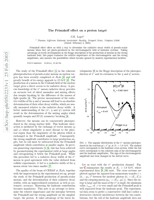
a r X i v :h e p -p h /0502233v 1 25 F eb 2005The Primakoffeffect on a proton targetget 11Thomas Jefferson National Accelerator Facility,Newport News,Virginia 23606(Dated:February 2,2008)Primakoffeffect offers us with a way to determine the radiative decay width of pseudo-scalar mesons when they are photo-produced in the electromagnetic field of hadronic systems.Taking advantage of recent developments in the Regge description of the production of mesons in the strong hadronic field,this paper evaluates the relative importance of the electromagnetic and the strong amplitudes,and assesses the possibilities which become opened by modern experimental facilities.PACS numbers:13.60.Le,12.40.NnThe study of the Primakoffeffect [1]in the coherent photoproduction of pseudo-scalar mesons on nuclear tar-gets has been recently completed at JLab [2]and will greatly benefit of its energy upgrade to 12GeV [3].The production of a meson in the Coulomb field of the nuclear target gives a direct access to its radiative decay.A pre-cise knowledge of the π◦meson radiative decay provides an accurate test of chiral anomalies and mixing effects due isospin breaking by the difference of the masses of light quarks [4].The precise measurement of the radia-tive widths of the ηand η′mesons will lead to an absolute determination of their other decay widths,which are usu-ally measured relative to the radiative decay width.A better understanding of the (π◦,ηand η′)system will result in the determination of the mixing angles which quantify isospin and SU(3)symmetry breaking [4].However,the mesons can be concurrently photopro-duced in the strong nuclear field.This hadronic inter-action is mediated by the exchange of vector mesons (ρand ω)whose singularity is more distant to the phys-ical region than the singularity of the photon which is exchanged in the Primakoffamplitude.Consequently,the strong amplitude contributes to large production an-gles,but its tail must be subtracted from the Primakoffamplitude which contributes at smaller angles.In previ-ous pioneering experiments [5,6],this has been achieved by parameterizing the experimental yield at large angles and extrapolating it below the Primakoffpeak.While this procedure led to a radiative decay width of the π◦meson in good agreement with the value deduced from collider experiments,it led to a radiative width of the ηmeson about two times smaller [7].The quality of the beam of CEBAF at JLab,together with the improvement in the experimental set-up,permit the study of the Primakoffproduction of pseudo-scalar mesons,and the determination of their radiative decay widths,with an unprecedented statistical,as well as sys-tematic,accuracy.Mastering the hadronic contribution becomes mandatory.This note is an attempt to deter-mine the relative importance and the interplay between the Primakoffand the strong amplitude on the simplest target,the proton.It takes advantage of the latest de-velopments [8]in the Regge description of the photopro-duction of π◦and its extension to the ηand η′sectors.1010110d σ/d t (µb /Ge V 2)FIG.1:duced in the reaction p (γ,π◦)p ,at E γ=5.8GeV.The dashed curve corresponds to the hadronic cross section,while the full curve corresponds to the coherent sum of the electromagnetic and the hadronic amplitudes.The sign of the electromagnetic amplitude has been changed in the dotted curve.Let us start with the π◦production channel.Fig-ure 1summarizes the results at E γ=5.8GeV,where experimental data [9,10]exist.The cross sections are plotted against the squared four-momentum transfer t =(k γ−p π◦)2between the incident photon (k γ=(E γ, kγ))and the outgoing meson (p π◦=(E π◦, p π◦)).Since the en-ergy is large and the mass of the π◦is small,the minimum value,t min ,of −t is very small and the Primakoffpeak is well separated from the hadronic peak.The experimen-tal data seem to prefer a constructive (full line)rather a destructive (dotted)interference between the two contri-butions,but the tail of the hadronic amplitude does not2 affect at all the Primakoffpeak in the range of small−twhere it dominates.Quantitatively,the hadronic amplitude is the same asin ref.[8],where its detailed expression and an extended discussion on the choice of the vertices and coupling con-stants can be found.Suffice to say that the amplitude is based on the exchange of the Regge trajectories of theρandωmesons,and takes into account the full spin-isospin structure of the electromagnetic and the strong vertices. We have chosen a degenerate Regge propagator for the ω,in order to accommodate for the minimum in the ex-perimental angular distribution around−t=0.5GeV2:Pω=(gµν−kµωkνωs◦αω(t)−1πα′ωΓ(αω(t))×1+exp[−iπαω(t)]m2ρ) s sin[παρ(t)]124m3V m2πg2Vπγ(5)This gives gωπγ=0.314,forΓω→πγ=720keV,and gρπγ=0.103,forΓρ→πγ=68keV[8].It turns out that the contraction between the mass dependent term kµρkνρ/m2ρof the vector meson propaga-tor and the electromagnetic vertex vanishes,and only the contribution of the gµνpart survives.Therefore, the Primakoffamplitude takes the same form as the vec-tor meson exchange amplitudes,provided that the Regge propagator is replaced by the Feynman propagator of the photonPγ=gµν16g2πγγ(7)The full curve in Figure1corresponds to the centralvalueΓπ→γγ=8eV of ref.[7](gπγγ=0.0114),while thedot-dashed curve uses8.4eV at the edge of the experi-mental values.Due to the structure of the electromagnetic vertices,both the hadronic amplitude and the Primakoffampli-tudes strickly vanish atθπ=0,and therefore t min.How-ever,the photon pole is so close to the physical regionthat it boosts the Primakoffamplitude orders of magni-tude above the strong amplitude.b1meson exchange may also contribute to the strongamplitude.In ref.[8]we found that,while it is necessaryto reproduce the beam asymmetry,it only modifies byabout10%the unpolarized cross section in the region ofthe minimum(−t∼0.5GeV2)and above.So it maymodify by the same amount the strong amplitude below−t∼10−3GeV2.Since our knowledge of its couplingconstants is on less solid ground than those ofρandωmesons,I do not retain its contribution.The model confirms the earlier estimate of the crosssection which was included in the experimental pa-pers[9,10].While there is no reason why the Primakoffamplitudes be different,the strong amplitude includedexchanges of theωand b1meson Regge trajectories andtheωPomeron cut,following refs.[11,12].The residuesof the poles werefitted to the data,contrary to the modelwhich I use:in ref.[8]we chose the values of strongand the electromagnetic coupling constants in the rangeof values determined in independent channels,and weimplemented the full spin-isospin structure of the lowermass realization of each Regge trajectory.In Figure1the experimental points have been plottedat the mean value of−t in each experimental bin inθπ◦.A new experimental determination of theπ◦Primakoffcross section,with a better angular resolution,is highlydesirable,especially in the domain where the Primakoffand the strong amplitudes interfere.Increasing the energy up to Eγ=9GeV does notchange dramatically the picture.As it can be seen in Fig-ure2,t min decreases by a factor two,but this does notimprove the separation between the Primakoffand thehadronic peak,which was already very good at5.8GeV.Note that the Regge model reproduces quite well the ex-perimental data[13]at this energy also.On the contrary,increasing the energy helps in theηandη′channels.Figure3shows the angular distributionof theηemitted in the p(γ,η)p reaction at Eγ=6GeV.The value of t min is more than two orders of magnitudebigger than in theπ◦channel.Consequently,one has torely on the tail of the Primakoffamplitude,which shows31010110d σ/d t (µb /Ge V 2)FIG.2:duced in the reaction p (γ,π◦)p ,at E γ=9GeV.The meaning of the curves is the same as in Fig.1.up above the tail of the strong amplitude.The model uses the same ρexchange amplitude (de-generate Regge propagator,eqs.3,with the same strong coupling constants)as in the π◦channel.The radiative coupling constant g ρηγ=0.81is deduced from the ex-perimental decay width Γρ→ηγ=39keV [7]with eq.5(where the πmass is replaced by the ηmass,m η).In the ωexchange amplitude,the radiative decay con-stant g ωηγ=0.29is also fixed by the experimental decay width Γω→ηγ=5.4keV [7].But,following ref.[14],I use the degenerate form,eq.3,instead of the non degen-erate form which I used in the π◦channel.The reason is that available experimental data [15]do not exhibit a minimum in the vicinity of the first node of the ωnon-degenerate Regge trajectory.In nature,Regge trajecto-ries (in the form of eq.1)go by pair,each having the same slope but a different signature,S =±1,when it connects members with either odd or even spins.When it hap-pens that each trajectory has the same,or comparable,coupling constants with the probe,they combine into a degenerate trajectory with or without a rotating phase (eq.3).Only experiment tells us what is the best choice.The conjecture is that the photon couples to a degener-ate trajectory of the ωin the ηphotoproduction channel,while it couples to a non-degenerate ωtrajectory in the π◦sector.Consequently the strong coupling constants of the omega are not necessarily the same in both channels.A good agreement with the data is achieved when I use g 2ωNN /4π=6.44and I keep κω=0.1010101101010101010-t GeV 2d σ/d t (µb /Ge V 2)FIG.3:The angular distribution of the ηmesons photopro-duced in the reaction p (γ,η)p ,at E γ=6GeV.The meaning of the curves is the same as in Fig.1.This set of coupling constants is different from the setof ref.[14]which has been obtained from a global fit in the ηand η′sector.I prefer to use a set which differs in a minimal way from the π◦sector set.It is worth to note that both sets lead to a similar accounting of the strong part of the cross section.The Primakoffcoupling constant of the ηmeson,g ηγγ=0.0429,is deduced from the average (includ-ing Primakoffmeasurement)value Γη→γγ=0.46keV of ref.[7]with the help of eq.7(where the πmeson mass is replaced by the ηmeson mass).The experimental study of the Primakoffeffect will greatly benefit of the increase of the incoming photon energy.Figure 4clearly demonstrates that,at E γ=11GeV,t min is lowered by about a factor three and the Primakoffpeak is clearly separated from the strong hadronic peak.Let us turn now to the η′channel,where I keep the same amplitudes as in the ηchannel and only change the radiative coupling constants.The η′radiative decay to the ρor the ωmesons is related to the radiative coupling constant in the following way:Γη′→V γ=αem (m 2η′−m 2V )3410-310-210-1110-610-510-410-310-210-1-t GeV 2d σ/d t (µb /Ge V 2)p(γ,η)pE γ = 11 GeVRegge ω+ρPrimakoffΓηγγ = 0.46 keVFIG.4:The angular distribution of the ηmesons photopro-duced in the reaction p (γ,η)p ,at E γ=11GeV.The meaning of the curves is the same as in Fig.1.Γη′→γγ=4.27keV of ref.[7]with the help of eq.7(where the πmeson mass is replaced by the η′meson mass).The results are shown in Figure 5at E γ=11GeV.Even at such a high energy,t min is high and the Pri-makoffcontribution appears as a shoulder on the tail of the strong amplitude.The situation is similar as in the ηsector at E γ=6GeV.Certainly an experiment with an excellent energy resolution will disentangle the Primakoffamplitude at the lowest angles,where it overwhelms by more that an order of magnitude the strong amplitude,which will be calibrated at higher angles.A measure-ment of ηmeson production at E γ=6GeV would be very welcome in this respect:it is already possible.Contrary to the π◦and the ηchannels,the experi-mental data set is extremely scarce.The model can only be compared to integrated experimental cross sec-tions [16,17].At E γ=5GeV,it predicts σ=0.1µb in the range of the experimental cross section σexp =0.17±0.12µb.This gives confidence in its extrapolation from the ηto the η′channel.But a more accurate deter-mination of the angular distribution is definitely needed.In conclusion,the Regge description of the strong hadronic amplitude has been extended from π◦to ηand η′photo-production.It reproduces all the available ex-perimental data and provides us with a solid starting point to evaluate the hadronic contribution below the Primakoffpeak.The Primakoffamplitude has been in-corporated in the model.While in the π◦sector it is prominent already at E γ=6GeV,its determination10-310-210-1110-610-510-410-310-210-1-t GeV 2d σ/d t (µb /Ge V 2)p(γ,η,)pE γ = 11 GeVRegge ω+ρPrimakoff Γη,γγ = 4.27 keVFIG.5:The angular distribution of the η′mesons photopro-duced in the reaction p (γ,η′)p ,at E γ=11GeV.The meaning of the curves is the same as in Fig.1.in the ηand η′sector requires accurate experiments at higher energies.I would like to thank A.Bernstein and R.Miskimen who triggered my interest in the Primakoffeffect,J.Goity who taught me its relevance to QCD and M.Van-derhaeghen for discussions on Regge models.[1]H.Primakoff,Phys.Rev.81,899(1951).[2]D.Dale et al.,PRIMEX Experiment,JLab-E-02-103.[3]Pre-Conceptual Design Report(pCDR)for the Scienceand Experimental Equipment for the 12GeV Upgrade of CEBAF (JLab,April 2003).[4]J.L.Goity,A.M.Bernstein and B.R.Holstein,Phys.Rev.D66,076014(2002).[5]A.Browman et al.,Phys.Rev.Lett.33,1400(1974).[6]A.Browman et al.,Phys.Rev.Lett.32,1067(1974).[7]S.Eidelman et al.,Phys.Lett.B572,1(2004).[8]M.Guidal,get and M.Vanderhaeghen,Nucl.Phys.A627,645(1997).[9]M.Braunschweig et al.,Phys.Lett.B26,405(1968).[10]M.Braunschweig et al.,Nucl.Phys.B20,191(1970).[11]J.P.Ader,M.Capdeville and Ph.Salin,Nucl.Phys.B3407(1967).[12]A.Capella and J.Tran Thanh Van,Nuovo Cimento Let-ters 1,321(1969).[13]R.Anderson et al.,Phys.Rev.D1,27(1970).[14]Wen-Tai Chiang et al.,Phys.Rev.C68,045202(2003).[15]W.Braunschweig et al.,Phys.Lett.B33,236(1970).[16]ABBHHM Collaboration,Phys.Rev.175,1669(1968).[17]W.Struczinski et al.,Nucl.Phys.B108,45(1976).。
SignalShark实时频谱分析监测接收器RF方向找器与定位系统说明书

The new generation in signal analysisReal-Time Spectrum AnalyzerMonitoring ReceiverRF Direction Finding andLocalization SystemMore and more devices have to share the available frequency spectrum as aresult of new technologies such as the Internet of things (IoT), machine tomachine (M2M) or car to car (C2C) communications, and the rapidly growing4G/5G mobile networks.It doesn’t matter whether you are making a wideband measurement of entirefrequency ranges, or searching for hidden signals, or needing to reliablydetect very short impulses, or localizing interference signals –SignalSharkgives you all the measurement solutions you need to cope with the increasinglycomplex radio frequency spectrum. Its design and excellent performance makeit ideal for on-site measurements as well as for fully-fledged laboratory use. SignalShark. Seven senses for signalsSignalShark –there’s a reason for the name. Just like its namesake, theSignalShark is an extremely efficient hunter, perfectly designed for its task.Its prey: interference signals. Its success rate: Exceptional. The real-timeanalyzer is a successful hunter, thanks to the interplay of its highly developedseven sensory functions. Seven senses that don’t miss a thing, and that makeit easy for you to identify and track down interferers in real-time./watch?v=pSZdR27j5LQ&t=14s• Frequency range: 8 kHz to 8 GHz• Weight: Approx. 4.1 kg / 9 lbs (with one battery)• Dimensions: 230 × 335 × 85 mm (9.06ʺ× 13.19ʺ× 3.35ʺ)Make it your deviceSignalShark is ready for the future, thanks toits many expansion facilities, and it can beoptimally adapted as needed to the widestvariety of applications.SignalShark – the 40 MHz real-timespectrum analyzerWhether you are in the lab or out in thefield, you will have the right analysis toolin hand with the SignalShark. You will beconvinced by its truly outstanding RF perfor-mance, as well as by its easily understood,application-oriented operating concept.The high real-time bandwidth with very highFFT overlapping ensures that you can reliablycapture even extremely brief and infrequentevents. The unusually fast scan rate results invery short measurement times even if youneed to cover wider frequency bands thanthe real-time bandwidth. Comprehensiveevaluation tools make sure that you canperform current and future measurementand analysis tasks up to laboratory instru-ment standards reliably, simply, and faster.SignalShark – the monitoring receiverThe extremely High Dynamic Range (HDR) ofthe SignalShark ensures that you can reliablydetect even the weakest signals in the pre-sence of very strong signals, and not confusethem with the artifacts of a normal receiver.This is a basic requirement for most tasksin the field of radio monitoring. Alongsidethe real-time spectrum analyzer, there is areceiver for audio demodulation, level mea-surement, and modulation analysis, whichcan be tuned to any frequency and channelbandwidth within the 40 MHz real-timebandwidth. And, if you need even more thanthe analysis tools of the SignalShark, you canprocess the I/Q data from the receiver exter-nally as a real-time stream and store themon internal or external data storage media.SignalShark – the direction findingand localization systemIt is often necessary to locate the positionof a signal transmitter once the signals havebeen detected and analyzed. SignalSharksupports the new Automatic Direction-Finding Antennas (ADFA) from Narda,allowing you to localize the source veryquickly and reliably. In fact, localization ischild’s play, thanks to the integrated mapsand localization firmware. Conveniently,homing-in using an ADFA mounted on amoving vehicle is also supported. Powerful,state of the art algorithms minimize theeffects of false bearings caused by reflectionsoff urban surroundings in real-time. Extre-mely light weight and easy to use manualdirection finding antennas are availablefor ”last mile“ localization.V I D E OVideo display port for external monitor or projector USB 2.0 for keyboard, mouse, printer, etc.fast, convenient measurementBuilt-in loudspeaker gives clear,loud sound reproduction, even in noisy environments/watch?v=0jqrwU_jPcsV I D E OSignalShark is a handy, portable, battery powered measuring device, yet it boasts performance that is otherwise only found in large, heavy laboratory grade equipment. It can be readily used instead of such expensive equipment because of its wide range of connection facilities and measurement functions.SignalShark –the real-time spectrum analyzer• HDR: extremely low noise and distortion, simultaneously • real-time bandwidth: 40 MHz – FFT overlap: 75 % (Fspan > 20 MHz)– FFT overlap: 87.5 % (Fspan ≤20 MHz, RBW ≤400 kHz))– FFT size: up to 16,384• Minimum signal duration for 100 % POI: 3.125 µs at full amplitude accuracy • Minimum detectable signal duration: < 5 ns • Persistence: up to 1.6 million spectrums per second • Spectrogram time resolution: down to 31.25 µs • Spectrogram detectors: up to three at the same time • RBW: 1 Hz - 800 kHz in real-time spectrum mode, 1 Hz - 6.25 MHz in scan spectrum mode• Filters conforming to CISPR and MIL for EMC measurements • Scan speed: Scan rate up to 50 GHz/s • Detectors: +Pk, RMS, Avg, -Pk, Sample• Markers: 8, additional noise power density and channel power function •Peak table: shows up to 50 highest spectral peaksReliable detection of extremely short and rare events in a 40 MHz real-time bandwidthA real-time analyzer calculates the spectrum by applying the FFT on overlapping time segments of the underlying I/Q data within its real-time bandwidth. The real-time band-width is only one of the key parameters for a real-time analyzer. The probability of inter-cept, POI, is easily just as important. This parameter describes the minimum time that the signal must be present for it to be always detected without any reduction in level. This time is affected by the maximum resolution bandwidth RBW and the FFT overlap. The SignalShark is a match for established laboratory analyzers with its minimum duration of 3.125 µsec for 100 %POI and full amplitude accuracy. The mini-mum detectable signal duration is < 5 nsec.SignalShark accomplishes this by a large signal immunity in combination with a very low intrinsic noise as well as a high FFT overlap and its large resolution bandwidth.That is outstanding for a hand-held analyzer. To accomplish this, SignalShark generally operates with an 87.5 % overlap, which is again outstanding for a hand-held analyzer.This means that even the shortest impulses are detected and the full signal to noise ratio is maintained for longer signals.Spectrogram shows more details than everWith SignalShark, you can use up to three detectors at the same time for the Spectrogram view. This makes it possible for you to easily visualize impulse inter-ference on broadcast signals and get much more information from the spectrogram. The extraordinarily fine time resolution of 31.25 µs means that you can completely reveal the time signatures of many signals.With the I/Q Analyzer option, you can resolve the spectrogram even more, to less than 200 ns.Persistence ViewA color display of the spectrum shows how often the displayed levels have occurred. This enables you to detect signals that would be masked by stronger signals in a normal spectrum view.=SignalShark is not just a very powerful real-time spectrum analyzer. It is also the ideal monitoring receiver, thanks to its near ITU-ideal spectrum monitoring dynamic capabilities, second receiver path and demodulators.SignalShark –the monitoring receiver• HDR: extremely low noise and distortion, simultaneously • CBW: 25 Hz - 40 MHz (Parks-McClellan, α= 0.16)• Filters for EMC measurements: CISPR, MIL • Detectors: +Pk, RMS, Avg, -Pk, Sample• EMC detectors: CPk, CRMS, CAvg (compliant with CISPR)• Level units: dBm, dB µV, dB(µV/m) …• Level uncertainty: < ±2dB • AFC• Audio demodulators: CW, AM, Pulse, FM, PM, LSB, USB, ISB, I/Q • AGC & squelch for audio demodulators • Modulation measurements: AM, FM, PM • I/Q streaming: Vita 49 (sample rate ≤25,6 MHz)• Remote control protocol: SCPIThe benefit of HDRThe extremely high dynamic range (HDR) of the SignalShark ensures that you can reliably detect even the weakest signals in the presence of very strong signals. The SignalShark’s pre-selector allows it to suppress frequencies that would other-wise interfere with the measurement. The excellent dynamic range of the SignalShark is the result of the ideal combination of the displayed averaged noise level (DANL)with the so-called large-signal immunity parameters, i.e. the second and third order intermodulation intercept points (IP 2and IP 3).It is important that these three factors are always specified for the same device setting (e.g. no attenuation, no pre-amplifier), as they vary considerably according to the setting.DDC 2, the additional receiver pathThe tuning frequency and the channel band-width of an additional receiver path, DDC 2,can be set independently from the real-time spectrum analyzer path, DDC 1, within the real-time bandwidth of the SignalShark. The I/Q data can be streamed to external devices in real-time, or they can be processed by the SignalShark itself for level measurements,audio demodulation, and modulation measurements. The very steep cutoffchannel filters capture 100 % of the signal in the selected channel without any degra-dation while completely suppressing the adjacent channels.CISPR compliant EMC detectors now also available for on-site applications The facility for selecting all the filters and detectors necessary for CISPR or MIL com-pliant EMC measurements is also available for the receiver as well as for the spectrum. If an interferer is detected, you can now decide on the spot whether or not the device needs to be taken out of service because of violating EMC regulations.EQDDC 1Overlap BufferFFT DetectorsPersist.Persistence StreamSpectrum StreamADC DataDDC 2DetectorsDetectorsI/Q BufferTrigger UnitDemodulatorsAGCLevel StreamDem. Det.StreamDem. Audio StreamAM & FM StreamI/Q StreamI 2+Q2I 2+Q2PATH 1PATH 2The block circuit diagram shows the two, independent digital down converters (DDC). These make it possible e.g. to observe the spectrum of the signal spectrum and demodulate it at the same time independently within the real-time bandwidth.Automatic Direction Finding Antenna ADFA 1 + 2Narda offers a large number of automatic and directional antennas for the SignalShark. Their unique characteristics combined with the SignalShark makes them unbeatable.Automatic Direction Finding Antenna ADFA 1The frequency range of ADFA 1 makes it particularly suitable for localizing interferers,e.g. in mobile communications networks:Frequency range: 200 MHz - 2.7 GHz Nine dipoles arranged on a 380 mm diameter circle for DFA central monopole is used as a reference element for DF or as an omnidirectional monitoring antennaBuilt-in phase shifter and switch matrix Direction finding method: correlative interferometerBearing uncertainty: 1° RMS (typ.)Built-in electronic compassBuilt-in GNSS receiver with antenna and PPS outputDiameter: 480 mmAutomatic Direction Finding Antenna ADFA 2 (available 2019)This ADFA is suitable for a wide range of localization tasks due to its wide frequency range:Frequency range: (500 kHz) 10 MHz -8 GHz Two crossed coils for DF at low frequencies Nine dipoles arranged on a 380 mm dia-meter circle for DF at medium frequencies Nine monopoles arranged on a 125 mm diameter circle for DF at high frequencies A central monopole is used as a reference element for DF or as an omnidirectional monitoring antennaBuilt-in phase shifter and switch matrix Direction finding method: Watson-Watt or correlative interferometerBearing uncertainty (10 MHz - 200 MHz): 2° RMS (typ.)Bearing uncertainty (200 MHz - 8 GHz): 1° RMS (typ.)Built-in electronic compassBuilt-in GNSS receiver with antenna and PPS output Diameter: 480 mm Automatic Direction Finding Antenna ADFA accessoriesConnecting cable, length 5 m or 15 m,low lossTripod including mounting accessories Mounting kit for magnetic attachment to a vehicle roofMounting kit for mast attachmentAfter you have localized the signal by SignalShark and ADFA using the car, you will need for last mile or to enter a building Narda’s handy, feather-light directional antennas and active antenna handle. They are the ideal choice in this situation. The antenna handle does more than just hold the antenna. Among other features, it has a built-in operating button that allows you to perform the main steps during manual direction finding, making the combination unbeatable.and take bearings on very weak or distant signals. The preamplifier gain is taken into account automatically when you make field strength or level measurements.The integrated operating button lets you make the main steps in the manual direction finding process.The following antennas to fit the antenna handle are available:• Loop Antenna: 9 kHz - 30 MHz• Directional Antenna 1: 20 MHz - 250 MHz • Directional Antenna 2: 200 MHz - 500 MHz • Directional Antenna 3: 400 MHz - 8 GHz A plug-in adapter with male N connector allows you to take advantage of the features of the handle even when you are using third-party antennas or external filters.Directional antenna 3400 MHz - 8 GHz350 g / 0.77 lbsDirectional antenna 1 20 MHz - 250 MHz 400 g / 0.88 lbs Loop antenna 9 kHz - 30 MHz 380 g / 0.84 lbs Directional antenna 2 200 MHz - 500 MHz 300 g / 0.66 lbs Active antenna handle with integrated compass and preamplifier 9 kHz - 8 GHz 470 g / 1.04 lbsAdapter,male N connectorN Antenna Elements0°90°180°270°Element SwitchReference Elementn1Quadrature Phase Shifter(Smart Antenna)+The Narda antenna handle and directional antennas are extremely light, making for fatigue-free signal searches.The convenient plug-in system allows you to change antennas very quickly.SignalShark recognizes the antenna and applies the appropriate antenna factors for field strength measurements automatically.SignalShark receives the azimuth,elevation and polarization of the antenna from the 3D electronic compass built into the handle, so manual direction finding could hardly be simpler.The preamplifier built into the handle is activated and deactivated bySignalShark, so you can further reduce SignalShark’s low noise figure to detectYou will often need to locate the position of a signal transmitter once thesignals have been detected or analyzed. SignalShark combined with Narda’snew automatic direction finding antennas (ADFA) and the very powerfulmap and localization firmware provides reliable bearings in the twinklingof an eye. The bearing results are processed by the SignalShark withoutneeding an external PC. Reliable localization of transmitters has not beenpossible before with so few hardware components.Transmitter localizationSignalShark simplifies transmitter localizationby autonomously evaluating all the availablebearing results and plotting them on a map,using a statistical distribution of bearinglines. The result is a so-called “heat map”,on which the possible location of the trans-mitter is plotted and color-coded accordingto probability. SignalShark also draws anellipse on the map centered on the estima-ted position of the transmitter and indicatingthe area where the transmitter has a 95 %probability of being located. The algorithmused by SignalShark to calculate the positionof an emitter is extremely powerful. It candetermine the position of the emitter bycontinuous direction finding when movingaround in a vehicle, even in a complexenvironment such as an inner-city area.The calculation is continuous inreal-time, so you can viewthe changing heat mapon the screen of theSignalShark andFast automatic direction findingSignalShark supports the new automaticdirection finding antennas (ADFA) fromNarda, which let you take a completebearing cycle in as little as 1.2 ms.The omnidirectional channel power and thespectrum are also measured during a bearingcycle, so you can monitor changes in thesignal level or spectrum concurrently withthe bearings. The AFDAs use differentantenna arrays, depending on the frequencyrange. At low frequencies, a pair of crossedcoils are used for the Watson-Watt methodof direction finding. At medium and highfrequencies, a circular array of nine dipolesor monopoles is used for the correlativeinterferometer direction finding method.SignalShark –The RF direction finding and localization system• Frequency range ADFA 1: 200 MHz - 2.7 GHz• Frequency range ADFA 2: 10 MHz - 8 GHz• Azimuth and elevation bearings• DF quality index• Complete bearing cycle: down to 1.2 ms• Omnidirectional level and spectrum during DF process• Uses OpenStreetMaps, other map formats can be imported• Easy to use, powerful map and localization software• The map and localization software runs on the handheldunit itselfThe SignalShark is a very powerful platform that Narda is continuously expanding. Options that will be available for delivery in 2019 are described below. Only the firmware of the SignalShark will be used to realize these options, which will be capable of on-site activation.High time resolution spectrogram HTRSalso available in the spectrum pathIn real-time spectrum mode, the ring buffer ofthe SignalShark records the I/Q data from thereal-time spectrum path rather than from thereceiver I/Q data. If you or a trigger eventhalts the real-time analyzer, the last up to200 million I/Q samples of the monitoredfrequency range are available. This correspondsto a timespan of at least 4 s, so you can zoomin on the spectrogram with a resolution ofbetter than 200 ns when the analyzer is halted.The FFT overlap can be up to 93.75 %, and nodetectors are needed that could reduce thetime resolution. You can even subsequentlyalter the RBW. The persistence view also adjustsso that it exactly summarizes the spectrumsin the time period covered by the zoomedsegment. This ensures that all the time orspectral details in the I/Q data can be madevisible. You can of course also save the I/Qdata of the zoomed segment.DF SpectrumThe SignalShark can find the directions ofseveral transmitters simultaneously in DFspectrum evaluation mode. This mode offersa persistence spectrum and a spectrogramof the azimuth in addition to the usual levelspectrum and spectrogram view. You canalso monitor frequency ranges that arewider than the real-time bandwidth of theSignalShark. You can distinguish betweendifferent transmitters much more easilythan before by means of DF spectrum mode,because the SignalShark shows you thedirection of incidence as well as the levelof each frequency bin.SignalShark I/Q analyzerSignalShark has a ring buffer for up to 200 million I/Q samples. The receiver I/Q data are normally written continuouslyto the ring buffer. The recording can be stopped by a trigger event. The recorded I/Q data are then transferred to the CPU of the SignalShark, where they are further processed.The following trigger sources are available: Frequency mask triggerReceiver levelExternal trigger sourceTimestampUser inputFree runThe following I/Q data views are available: I and Q versus timeMagnitude versus time (Zero-span) Vector diagramHigh time resolution spectrogram Persistence You can of course also save the I/Q data as adata set, and you can even stream the datadirectly to permanent storage media in orderto make very long recordings of the I/Q data.You can then replay such long-term recor-dings using the integrated I/Q analyzer, orprocess them externally.2 x 10 MHz LTE signal recorded in a HTRS. Time resolution1 µs. The extremely high time resolution renders the signaltransparent at low traffic levels (right), so you can spotpossible interference within the frame structure.More Information about technical details andaccessories like transport case and car chargerunit can be found in the SignalShark data sheet./en/signalsharkNarda is a leading supplier …N S T S 06/18 E 0333A T e c h n i c a l a d v an c e s , e r r o r s a n d o m i s s i o n s e x c l u d e d .© N a r d a S a f e t y T e s t S o l u t i o n s 2014. ® T h e n a m e a n d l o g o a r e t h e r e g i s t e r e d t r a d e m a r k s o f N a r d a S a f e t y T e s t S o l u t i o n s G m b H a n d L 3 C o m m u n i c a t i o n s H o l d i n g s , I n c .—T r a d e n a m e s a r e t h e t r a d e m a r k s o f t h e i r o w n e r s .r o e n e r -d e s i g n .d eNarda Safety Test Solutions 435 Moreland RoadHauppauge, NY11788, USA Phone +1 631 231-1700Fax +1 631 231-1711**************************… of measuring equipment in the RF test and measurement, EMF safety and EMC sectors. The RF test and measurement sector covers analyzers and instruments for measuring andidentifying radio sources. The EMF safety product spectrum includes wideband and frequency-selective measuring devices, and monitors for wide area coverage or which can be worn on the body for personal safety. The EMC sector offers instruments for determining the electro-magnetic compatibility of devices under the PMM brand. The range of services includes servicing, calibration, accredited calibration, and continuous training programs.Narda Safety Test Solutions GmbH Sandwiesenstraße 772793 Pfullingen, Germany Tel. +49 7121 97 32 0Fax +49 7121 97 32 790********************* /en/signalshark。
如何询问稿件及编辑答复

如何询问稿件及编辑答复!Dear Editor,I'm not sure if it is the right time to contact you again to inquire about the status of my submittedmanuscript(ref:****) although nearly one month have passed since I contacted you last time. Iwould be greatly appreciate ifyou could spend some of your time check the status for me.Best regards***老外的答复:Dear ***,Thank you for your e-mail. We would like to sincerely apologise for the long delay in reviewingyour article. Your article was sent to many different referees, most of whom felt that they wereeither unqualified or their time was too restricted to review the paper. We understand that youmust feel frustrated, and we are sorry for this. Please understand that we rely entirely on thereferee‟s to return articles to us sp eedily. Unfortunately, this is not always the case. It would bemuch appreciated if you could suggest an alternative referee for your article, a person who may beable to review the article in a more appropriate time frame. Please forward this person's contactdetails (e-mail address) to us as soon as possible. We will do our very best to speed up the process.We apologize for any inconvenience that you experienced due to this delay, and we appreciateyour understanding and tried patience in this regard.邀请函上没有老外签名,无法签证背景介绍:老外的签名跟我们的盖章查不多,没有签名的东西是不正式的,我去参加某次国际会议,签证的时候才发现,粗心的老外给我的邀请函没有他的签名,我只好email 给她询问,并要求马上传真给我。
Measurement of the Branching Fractions of $Lambda_{c}^{+}to pbar{K}n(pi)$
a rXiv:h ep-e x /97912v11Sep1997CLNS 97/1502CLEO 97-18Measurement of the Branching Fractions of Λ+c →p K 0,p K 0π0,all measured relative to pK −π+.The relative branching fractions are 0.67±0.04±0.11,0.46±0.02±0.04,0.52±0.04±0.05,and 0.66±0.05±0.07respectively.M.S.Alam,1S.B.Athar,1Z.Ling,1A.H.Mahmood,1H.Severini,1S.Timm,1F.Wappler,1A.Anastassov,2J.E.Duboscq,2D.Fujino,2,∗K.K.Gan,2T.Hart,2 K.Honscheid,2H.Kagan,2R.Kass,2J.Lee,2M.B.Spencer,2M.Sung,2A.Undrus,2,†R.Wanke,2A.Wolf,2M.M.Zoeller,2B.Nemati,3S.J.Richichi,3W.R.Ross,3P.Skubic,3 M.Bishai,4J.Fast,4J.W.Hinson,4N.Menon,ler,4E.I.Shibata,4I.P.J.Shipsey,4M.Yurko,4L.Gibbons,5S.Glenn,5S.D.Johnson,5Y.Kwon,5,‡S.Roberts,5E.H.Thorndike,5C.P.Jessop,6K.Lingel,6H.Marsiske,6M.L.Perl,6 D.Ugolini,6R.Wang,6X.Zhou,6T.E.Coan,7V.Fadeyev,7I.Korolkov,7Y.Maravin,7 I.Narsky,7V.Shelkov,7J.Staeck,7R.Stroynowski,7I.Volobouev,7J.Ye,7M.Artuso,8 A.Efimov,8M.Goldberg,8D.He,8S.Kopp,8G.C.Moneti,8R.Mountain,8S.Schuh,8 T.Skwarnicki,8S.Stone,8G.Viehhauser,8X.Xing,8J.Bartelt,9S.E.Csorna,9V.Jain,9,§K.W.McLean,9S.Marka,9R.Godang,10K.Kinoshita,i,10P.Pomianowski,10 S.Schrenk,10G.Bonvicini,11D.Cinabro,11R.Greene,11L.P.Perera,11G.J.Zhou,11B.Barish,12M.Chadha,12S.Chan,12G.Eigen,ler,12C.O’Grady,12M.Schmidtler,12J.Urheim,12A.J.Weinstein,12F.W¨u rthwein,12D.W.Bliss,13G.Masek,13H.P.Paar,13S.Prell,13V.Sharma,13D.M.Asner,14J.Gronberg,14T.S.Hill,nge,14S.Menary,14R.J.Morrison,14H.N.Nelson,14T.K.Nelson,14C.Qiao,14J.D.Richman,14D.Roberts,14A.Ryd,14M.S.Witherell,14R.Balest,15B.H.Behrens,15W.T.Ford,15H.Park,15J.Roy,15J.G.Smith,15J.P.Alexander,16C.Bebek,16B.E.Berger,16K.Berkelman,16K.Bloom,16D.G.Cassel,16H.A.Cho,16D.S.Crowcroft,16M.Dickson,16P.S.Drell,16K.M.Ecklund,16R.Ehrlich,16A.D.Foland,16P.Gaidarev,16B.Gittelman,16S.W.Gray,16D.L.Hartill,16B.K.Heltsley,16P.I.Hopman,16J.Kandaswamy,16P.C.Kim,16D.L.Kreinick,16 T.Lee,16Y.Liu,16G.S.Ludwig,16N.B.Mistry,16C.R.Ng,16E.Nordberg,16M.Ogg,16,∗∗J.R.Patterson,16D.Peterson,16D.Riley,16A.Soffer,16B.Valant-Spaight,16C.Ward,16 M.Athanas,17P.Avery,17C.D.Jones,17M.Lohner,17C.Prescott,17J.Yelton,17J.Zheng,17G.Brandenburg,18R.A.Briere,18A.Ershov,18Y.S.Gao,18D.Y.-J.Kim,18 R.Wilson,18H.Yamamoto,18T.E.Browder,19F.Li,19Y.Li,19J.L.Rodriguez,19T.Bergfeld,20B.I.Eisenstein,20J.Ernst,20G.E.Gladding,20G.D.Gollin,20 R.M.Hans,20E.Johnson,20I.Karliner,20M.A.Marsh,20M.Palmer,20M.Selen,20 J.J.Thaler,20K.W.Edwards,21A.Bellerive,22R.Janicek,22D.B.MacFarlane,22P.M.Patel,22A.J.Sadoff,23R.Ammar,24P.Baringer,24A.Bean,24D.Besson,24D.Coppage,24C.Darling,24R.Davis,24N.Hancock,24S.Kotov,24I.Kravchenko,24N.Kwak,24S.Anderson,25Y.Kubota,25S.J.Lee,25J.J.O’Neill,25S.Patton,25R.Poling,25T.Riehle,25V.Savinov,25and A.Smith251State University of New York at Albany,Albany,New York122222Ohio State University,Columbus,Ohio432103University of Oklahoma,Norman,Oklahoma730194Purdue University,West Lafayette,Indiana479075University of Rochester,Rochester,New York146276Stanford Linear Accelerator Center,Stanford University,Stanford,California94309 7Southern Methodist University,Dallas,Texas752758Syracuse University,Syracuse,New York132449Vanderbilt University,Nashville,Tennessee3723510Virginia Polytechnic Institute and State University,Blacksburg,Virginia24061 11Wayne State University,Detroit,Michigan4820212California Institute of Technology,Pasadena,California9112513University of California,San Diego,La Jolla,California9209314University of California,Santa Barbara,California9310615University of Colorado,Boulder,Colorado80309-039016Cornell University,Ithaca,New York1485317University of Florida,Gainesville,Florida3261118Harvard University,Cambridge,Massachusetts0213819University of Hawaii at Manoa,Honolulu,Hawaii9682220University of Illinois,Champaign-Urbana,Illinois6180121Carleton University,Ottawa,Ontario,Canada K1S5B6and the Institute of Particle Physics,Canada22McGill University,Montr´e al,Qu´e bec,Canada H3A2T8and the Institute of Particle Physics,Canada23Ithaca College,Ithaca,New York1485024University of Kansas,Lawrence,Kansas6604525University of Minnesota,Minneapolis,Minnesota55455Since thefirst observation of the lowest lying charmed baryon,theΛ+c,there have been many measurements made of its exclusive decay channels.As it is difficult to measure the production cross-section of theΛ+c baryons,decay rates are typically presented as branching ratios relative toΛ+c→pK−π+,the most easily observed decay channel.However,fewer than half of theΛ+c hadronic decays are presently accounted for.Measurement of these modes is of practical as well as theoretical interest.Here,we present measurements of the branching fractions ofΛ+c into pK−π+π0,p K0π+π−,and pE2beam−m2Λc is the scaled momentum of theΛ+c candidate.Approximately 60%ofΛ+c baryons from cK0candidates were identified in their decay K0s→π+π−,by reconstructing a secondary vertex from the intersection of two oppositely charged tracks in the r−φplane. The invariant mass of theMode MC Width(MeV)SignalK0191025±40 pK0π027774±52 TABLE I.The number ofΛ+c’s found with x p(Λc)>0.5D∗+→K−π+π+decays that were identified topologically.The reconstruction efficiency of theΛ+c decays has some dependence on the resonant substructure of these states.In the case of the pK−π+mode,the Monte-Carlo generator produced a mixture of non-resonant three-body decay together with∆++K−and pK0→K0s and K0s→π=π−branching fractions.We have considered many possible sources of systematic error in the measurement.The main contributors to the systematic uncertainty came from the following sources:1)Un-certainties in thefitting procedures,which were estimated by looking at the changes in the yields using different orders of polynomial background and different signal widths(15%in the case of pK−π+π0,but much smaller for the other modes),2)uncertainties due to the unknown mix of resonant substructure in the multi-body decays(up to3%depending on the mode),3)uncertainties due toπ0finding(5%),K0sfinding(5%)and trackfinding(1%), and4)uncertainties in the reconstruction efficiency due to the particle identification criteria for protons and kaons(4%).These uncertainties have been added in quadrature to obtain the total systematic uncertainty for each mode,taking into account the fact that many of these tend to cancel in a measurement of ratios of branching fractions.There are three main types of quark decay diagrams that contribute toΛ+c decays.The simplest method is the simple spectator diagram in which the virtual W+fragments inde-pendently of the spectator quark.The second method involves the quark daughters of the W+combining with the remaining quarks.The third method,W-exchange,involves the W+ combining with the initial d quark.Unfortunately all the decay modes under investigation here can proceed by more than one of these decay diagrams,and their decay rates are not amenable to calculation.In conclusion,we have measured new branching fractions of theΛ+c into4decay modes, measured relative to the normalizing modeΛ+c→pK−π+.The results for three of these modes are in agreement with,and more accurate than,previous measurements.We have made thefirst measurement of the decay rate ofΛ+c→pMode Relative Efficiency B/B(pK−π+)Previous MeasurementsK00.2180.46±0.02±0.040.44±0.07±0.05[4]0.55±0.17±0.14[6]0.62±0.15±0.03[7]pK0π00.1150.66±0.05±0.07TABLE II.The measured relative branching fractionsREFERENCES[1]Y.Kubota et al.,Nucl.Inst.and Methods A320,66(1992).[2]R.Brun et al.,CERN/DD/EE/84-11.[3]Review of Particle Properties,R.Barnett et al.,Phys.Rev.D541(1996).[4]P.Avery et al.,Phys.Rev.D43,3499(1991)[5]S.Barlag et al.,Z.Phys.C48,29(1990).[6]J.Anjos et al.,Phys.Rev.D41,801(1990).[7]H.Albrecht et al.,Phys.Lett.B207,109(1988).IVeM5/stnevEIMass (GeV)FIG.1.Invariant mass plots for the5different decay modes of theΛ+c。
Early-universe constraints on a Primordial Scaling Field
a r X i v :a s t r o -p h /0104162v 2 28 M a y 2001Early-universe constraints on Dark EnergyRachel Bean ♯,Steen H.Hansen ♭and Alessandro Melchiorri ♭♯Theoretical Physics,The Blackett Laboratory,Imperial College,Prince Consort Road,London,U.K.♭NAPL,University of Oxford,Keble road,OX13RH,Oxford,UK In the past years ’quintessence’models have been considered which can produce the accel-erated expansion in the universe suggested by recent astronomical observations.One of the key differences between quintessence and a cosmological constant is that the energy density in quintessence,Ωφ,could be a significant fraction of the overall energy even in the early uni-verse,while the cosmological constant will be dynamically relevant only at late times.We use standard Big Bang Nucleosynthesis and the observed abundances of primordial nuclides to put constraints on Ωφat temperatures near T ∼1MeV .We point out that current ex-perimental data does not support the presence of such a field,providing the strong constraint Ωφ(MeV)<0.045at 2σC.L.and strengthening previous results.We also consider the effect a scaling field has on CMB anisotropies using the recent data from Boomerang and DASI,providing the CMB constraint Ωφ≤0.39at 2σduring the radiation dominated epoch.Introduction.Recent astronomical observations [1]suggest that the energy density of the universe is dominated by a dark energy component with nega-tive pressure which causes the expansion rate of the universe to accelerate.One of the main goals for cos-mology,and for fundamental physics,is ascertaining the nature of the dark energy [2].In the past years scaling fields have been con-sidered which can produce an accelerated expansion in the present epoch.The scaling field is known as “quintessence”and a vast category of “tracker”quintessence models have been created (see for exam-ple [3,4]and references therein),in which the field approaches an attractor solution at early times,with its energy density scaling as a fraction of the domi-nant component.The desired late time accelerated expansion behaviour is then set up independently of initial conditions,with the quintessential field domi-nating the energy content.Let us remind the reader of the two key differ-ences between the general quintessential model and a cosmological constant:firstly,for quintessence,the equation-of-state parameter w φ=p/ρvaries in time,usually approaching a present value w 0<−1/3,whilst for the cosmological constant remains fixed at w Λ=−1.Secondly,during the attractor regime the energy density in quintessence Ωφis,in general,a sig-nificant fraction of the dominant component whilst ΩΛis only comparable to it at late times.Future supernovae luminosity distance data,as might be obtained by the proposed SNAP satel-lite,will probably have the potential to discriminate between different dark energy theories [5].These datasets will only be able to probe the late time be-haviour of the dark energy component at red-shift z <2,however.Furthermore,since the luminosity distance depends on w through a multiple integral re-lation,it will be difficult to infer a precise measure-ment of w (z )from these datasets alone [6].In this Letter we take a different approach to the problem,focusing our attention on the early time be-haviour of the quintessence field,when the trackingregime is maintained in a wide class of models,and Ωφis a significant (≥0.01,say)fraction of the overall density.In particular,we will use standard big bang nucle-osynthesis and the observed abundances of primordial nuclides to put constraints on the amplitude of Ωφat temperatures near T ∼1MeV.The inclusion of a scaling field increases the expansion rate of the uni-verse,and changes the ratio of neutrons to protons at freeze-out and hence the predicted abundances of light elements.The presence of this field in the radiation domi-nated regime also has important effects on the shape of the spectrum of the cosmic microwave background anisotropies.We use the recent anisotropy power spectrum data obtained by the Boomerang [7]and DASI [8]experiments to obtain further,independent constraints on Ωφduring the radiation dominated epoch.There are a wide variety of quintessential models;we limit our analysis to the most general ones,with attractor solutions established well before nucleosyn-thesis.More specifically,we study a tracker model based on the exponential potential V =V 0e −λφ[9].If the dominant component scales as ρn =ρ0(a 0λ2.However,the pure exponential potential,since it simply mimics the scaling of the dominant matter in the attractor regime,cannot produce an ac-celerated expanding universe in the matter dominated epoch.Therefore,we focus our attention on a recently pro-posed model by Albrecht and Skordis (referred to as the AS model from herein)[10],motivated by physics in the low-energy limit of M-theory,which includes a factor in front of the exponential,so that it takes the form V =V 0 (φ0−φ)2+A e−λφ.The prefactor introduces a small minimum in the potential.When the potential gets trapped in this minimum its kinetic energy disappears,triggering a period of accelerated-1.0-0.8-0.6-0.4-0.20.0-1.0-0.8-0.6-0.4-0.20.00.2-1.0-0.8-0.6-0.4-0.20.00.2log 10(a)w t o tlog 10(a)ΩQFIG.1.Top panel:Time behaviour of the fractional energy density Ωφfor the Albrecht and Skordis model to-gether with the constraints presented in the paper.The parameters of the models are (assuming h =0.65and Ωφ=0.65)λ=3,φ0=87.089,A =0.01and λ=8,φ0=25.797,A =0.01.Bottom panel:Time behaviour for the overall equation of state parameter w tot for the two models.Luminosity distance data will not be useful in differentiating the two models.expansion,which never ends if Aλ2<1[11].In Fig.1we introduce and summarise the main re-sults of the paper.In the figure,the BBN constraints obtained in section 2,and the CMB constrains ob-tained in section 3are shown together with two dif-ferent versions of the AS model which both satisfy the condition Ωφ=0.65today.Constraints from BBN.In the last few years impor-tant experimental progress has been made in the mea-surement of light element primordial abundances.For the 4He mass fraction,Y He ,two marginally compati-ble measurements have been obtained from regression against zero metallicity in blue compact galaxies.A low value Y He =0.234±0.003[12]and a high one Y He =0.244±0.002[13]give realistic bounds.We use the high value in our analysis;if one instead con-sidered the low value,the bounds obtained would be even stronger.Observations in different quasar absorption line sys-tems give a relative abundance for deuterium,critical in fixing the baryon fraction,of D/H =(3.0±0.4)·10−5[14].Recently a new measurement of deuterium in the damped Lyman-αsystem was presented [15],leading to the weighted abundance D/H =(2.2±0.2)·10−5.We use the value from [14]in our analysis;the use of [15]leads to even stronger bound.In the standard BBN scenario,the primordial abun-dances are a function of the baryon density η∼Ωb h 2only.To constrain the energy density of a primor-FIG. 2.1,2and 3σlikelihood contours in the (Ωb h 2,Ωφ(1MeV))parameter space derived from 4He and D abundances.dial field a T ∼MeV,we modified the standard BBN code [16],including the quintessence energy compo-nent Ωφ.We then performed a likelihood analysis in the parameter space (Ωb h 2,ΩBBN φ)using the observed abundances Y He and D/H .In Fig.2we plot the 1,2and 3σlikelihood contours in the (Ωb h 2,ΩBBN φ)plane.Our main result is that the experimental data for 4He and D does not favour the presence of a dark energy component,providing the strong constraint Ωφ(MeV)<0.045at 2σ(corresponding to λ>9for the exponential potential scenario),strengthening sig-nificantly the previous limit of [17],Ωφ(MeV)<0.2.The reason for the difference is due to the improve-ment in the measurements of the observed abun-dances,especially for the deuterium,which now corre-sponds to approximately ∆N eff<0.2−0.3additional effective neutrinos (see,e.g.[18]),whereas Ref.[17]used the conservative value ∆N eff<1.5.One could worry about the effect of any underesti-mated systematic errors,and we therefore multiplied the error-bars of the observed abundances by a factor of 2.Even taking this into account,there is still a strong constraint Ωφ(MeV)<0.09(λ>6.5)at 2σ.Constraints from CMB.The effects of a scaling field on the angular power spectrum of the CMB anisotropies are several [10].Firstly,if the energy den-sity in the scaling quintessence is significant during the radiation epoch,this would change the equality redshift and modify the structure of the peaks in the CMB spectrum (see e.g.[19]).Secondly,since the inclusion of a scaling field changes the overall content in matter and energy,the angular diameter distance of the acoustic horizon size at recombination will change.This would result in a shift of the peak positions on the angular spectrum.It is important to note that this effect does not quali-tatively add any new features additional to those pro-01002003004005006007008009001000110020406080100FIG.3.CMB anisotropy power spectra for the Al-brecht-Skordis models with λ=3,φ0=87.22and A =0.009(long dash),λ=8,φ0=32.329and A =0.01(short dash)(both with Ωφ=0.65and h =0.65),and a cosmological constant with ΩΛ=0.65,N ν=3.04(full line)and N ν=7.8(dash-dot).duced by the presence of a cosmological constant [20].Third,the time-varying Newtonian potential after decoupling will produce anisotropies at large angu-lar scales through the Integrated Sachs-Wolfe (ISW)effect.Again,this effect will be difficult to disentan-gle from the same effect generated by a cosmologi-cal constant,especially in view of the affect of cos-mic variance and/or gravity waves on the large scale anisotropies.Finally,the perturbations in the scaling field about the homogeneous solution will also slightly affect the baryon-photon fluid modifying the structure of the spectral peaks.However,this effect is generally neg-ligible.From these considerations,supported also by re-cent CMB analysis [21,22],we can conclude that the CMB anisotropies alone cannot give significant con-straints on w φat late times.If,however,Ωφis signif-icant during the radiation dominated epoch it would leave a characteristic imprint on the CMB spectrum.The CMB anisotropies can then provide a useful cross check on the bounds obtained from BBN.To obtain an upper bound on Ωφat last scatter-ing,we perform a likelihood analysis on the recent Boomerang [7]and DASI [8]data.The anisotropy power spectrum from BOOMERang and DASI was estimated in 19bins between ℓ=75and ℓ=1025and in 9bins,from ℓ=100to ℓ=864respec-tively.Our database of models is sampled as in [23],we include the effect of the beam uncertainties for the BOOMERanG data and we use the public available covariance matrix and window functions for the DASI experiment.There are naturally degeneracies between Ωm and ΩΛwhich are broken by the inclusion of SN1a data [1].0.010.111001000FIG.4.Matter power spectra for 3models in fig. 3.The predictions support those in the CMB spectra,the quintessence model in agreement with BBN λ=8(short dash)mimics the ΩΛ=0.65spectrum with N ν=3.0(full line).The model with λ=3(long dash)is in clear dis-agreement with observations.By finding the remaining “nuisance”parameters which maximise the likelihood,we obtain Ωφ<0.39at 2σlevel during the radiation dominated epoch.Therefore,while there is no evidence from the CMB anisotropies for a presence of a scaling field in the ra-diation dominated regime,the bounds obtained are actually larger than those from BBN.In Fig.3we plot the CMB power spectra for 4alter-native scenarios.The CMB spectrum for the model which satisfies the BBN constraints is practically in-distinguishable from the spectrum obtained with a cosmological constant.Nonetheless,if the dark energy component during radiation is significant,the change in the redshift of equality leaves a characteristic im-print in the CMB spectrum,breaking the geometri-cal degeneracy.This is also found when considering non-minimally coupled scalar fields [24],even when the scalar is a small fraction of the energy density at last scattering.In the minimally coupled models con-sidered here,this is equivalent to an increase in the neutrino effective number,i.e.altering the number of relativistic degrees of freedom at last scattering.In Fig.4we have plotted the corresponding mat-ter power spectra together with the decorrelated data points of Ref.[25].As one can see,the model with λ=3is in disagreement with the data,producing less power than the model with λ=8,with this last one still mimicking a cosmological constant.The less power can be still explained by the increment in the radiation energy component which shift the equality at late time and the position of the turn-around in the matter spectrum towards larger scales.A bias fac-tor could in principle solve the discrepancy between the λ=3model and the data,however,the mat-ter fluctuations over a sphere of size 8h −1Mpc areσ8∼0.5to be compared with theobserved valueσ8=0.56Ω−0.47m ∼0.9[26].Weak lensing observa-tions[27]may open up further opportunities to con-strain quintessence models even more tightly through the matter power spectrum.Conclusions.We have examined BBN abundances and CMB anisotropies in a cosmological scenario with a scalingfield.We have quantitatively discussed how large values of the fractional density in the scal-ingfieldΩφat T∼1MeV can be in agreement with the observed values of4He and D,assuming standard Big Bang Nucleosynthesis.The2σlimit Ωφ(1MeV)<0.05severely constrains a wide class of quintessential scenarios,like those based on an expo-nential potential.For example,for the pure expo-nential potential the total energy today is restricted toΩφ=3[1]P.M.Garnavich et al,Ap.J.Letters493,L53-57(1998);S.Perlmutter et al,Ap.J.483,565(1997);S.Perlmutter et al(The Supernova Cosmology Project), Nature39151(1998);A.G.Riess et al,Ap.J.116, 1009(1998);B.P.Schmidt,Ap.J.507,46-63(1998).[2]N.Bahcall,J.P.Ostriker,S.Perlmutter andP.J.Steinhardt,Science284,1481(1999)[astro-ph/9906463]; A.H.Jaffe et al,Phys.Rev.Lett.86 (2001)[astro-ph/0007333].[3]I.Zlatev,L.Wang,&P.Steinhardt,Phys.Rev.Lett.82896-899(1999).[4]P.Brax,J.Martin&A.Riazuelo,Phys.Rev.D.,62103505(2000).[5]J.Weller, A.Albrecht,Phys.Rev.Lett.861939(2001)[astro-ph/0008314];T.Chiba,T.Nakamura, Phys.Rev.D62(2000)121301,[astro-ph/0008175];D.Huterer and M.S.Turner,[astro-ph/0012510];M.Tegmark,[astro-ph/0101354];V.Barger, D.Marfatia Phys.Lett.B498(2001)67-73,[astro-ph/0009256].[6]I.Maor,R.Brustein and P.J.Steinhardt,Phys.Rev.Lett.86,6(2001)[astro-ph/0007297].[7]terfield et al.,astro-ph/0104460.[8]C.Pryke et al.,astro-ph/0104489.[9]J.J.Halliwell,Phys.Lett.B185341(1987);J.Bar-row,Phys.Lett.B18712(1987);B.Ratra,P.Pee-bles,Phys.Rev.D373406(1988);C.Wetterich,As-tron.&Astrophys.301321(1995).[10]A.Albrecht,C.Skordis,Phys.Rev.Lett.842076(2000)[astro-ph/9908085]; C.Skordis,A.Albrect,Phys.Rev.D,Submitted[astro-ph/0012195].[11]J.Barrow,R.Bean,J.Maguejo(2000)[astro-ph/0004321].[12]K.A.Olive and G.Steigman,Astrophys.J.Suppl.Ser.97,49(1995).[13]Y.I.Izotov and T.X.Thuan,ApJ,500188(1998);[14]S.Burles and D.Tytler,ApJ,499689(1998).[15]M.Pettini and D.V.Bowen,[astro-ph/0104474].[16]L.Kawano,Fermilab-Pub-92/04-A(1992).[17]P.G.Ferreira and M.Joyce,Phys.Rev.Lett.79(1997)4740-4743[astro-ph/9707286];P.G.Ferreira and M.Joyce,Phys.Rev.D58(1998)023503[astro-ph/9711102].[18]S.Burles,K.M.Nollett,J.N.Truran andM.S.Turner,Phys.Rev.Lett.82,4176(1999)[astro-ph/9901157];S.Esposito,G.Mangano,G.Miele and O.Pisanti,JHEP0009(2000)038[astro-ph/0005571].[19]W.Hu,D.Scott,N.Sugiyama and M.White,Phys.Rev.D52(1995)5498[astro-ph/9505043].[20]G.Efstathiou&J.R.Bond[astro-ph/9807103].[21]A.Balbi,C.Baccigalupi,S.Matarrese,F.Perrottaand N.Vittorio,Astrophys.J.547(2001)L89[astro-ph/0009432].[22]J.R.Bond et al.[The MaxiBoom Collaboration],astro-ph/0011379.[23]S.Esposito,G.Mangano,A.Melchiorri,G.Miele andO.Pisanti,Phys.Rev.D63(2001)043004[astro-ph/0007419].[24]R.Bean,[astro-ph/0104464][25]A.J.S.Hamilton&M.Tegmark,[astro-ph/0008392].[26]Viana P.,Liddle A.R.,1999,MNRAS,303,535.[27]Van Waerbeke L.et al.,[astro-ph/0101511][28]A. D.Dolgov,S.H.Hansen,S.Pastor andD.V.Semikoz,Nucl.Phys.B548(1999)385[hep-ph/9809598].[29]P.Di Bari and R.Foot,Phys.Rev.D63(2001)043008[hep-ph/0008258].[30]S.Dodelson,M.Kaplinghat and E.Stewart,Phys.Rev.Lett.85(2000)5276[astro-ph/0002360]. [31]M.Zaldarriaga&U.Seljak,ApJ.469437(1996).。
Measurements of High Density Matter at RHIC

∗
pmjacobs@
1
1 Introduction
At high temperature or baryon density, hadronic matter dissolves into a soup of its constituent quarks and gluons. For an asymptotically free field theory such as QCD, the state of matter at high energy density is simple1: long range (low momentum) interactions are screened, and short range (high momentum) interactions are weak, leading to an ideal gas equation of state in the high energy density limit. At temperature T ≫ ΛQCD matter is a gas of deconfined, weakly interacting quarks and gluons (the fined and matter consists of strongly interacting hadrons. “Quark-Gluon Plasma”, or QGP), whereas at T ≪ ΛQCD quarks and gluons are con-
temperature QCD can only be carried out numerically on the lattice.3 Fig. 2 shows a recent lattice calculation of the energy density ǫ as function of temperature for twoand three-flavor QCD. ǫ exhibits a sharp rise in the vicinity of the critical temperature TC , indicating a rapid change in the density of underlying degrees of freedom. The ideal gas Stefan-Boltzmann limit ǫSB has not yet been achieved at T ∼ 4TC . Putting in physGeV/fm3 . This value should be kept in mind for comparison to conditions achieved in laboratory experiments. The order of the deconfinement phase transition can be determined in some limiting cases.3 It is first order for pure gauge and for three light quarks, second order for two light and one heavy quark. For physical quark masses the order of the transition, or 2 ical values, TC ∼ 175 MeV, resulting in critical energy density ǫC = (6 ± 2)TC 4 ∼ 1
Discrete Applied Mathematics

Discrete Applied Mathematics157(2009)2217–2220Contents lists available at ScienceDirectDiscrete Applied Mathematicsjournal homepage:/locate/damPreface$This special issue on Networks in Computational Biology is based on a workshop at Middle East Technical University in Ankara,Turkey,September10–12,2006(.tr/Networks_in_Computational_Biology/). Computational biology is one of the many currently emerging areas of applied mathematics and science.During the last century,cooperation between biology and chemistry,physics,mathematics,and other sciences increased dramatically,thus providing a solid foundation for,and initiating an enormous momentum in,many areas of the life sciences.This special issue focuses on networks,a topic that is equally important in biology and mathematics,and presents snapshots of current theoretical and methodological work in network analysis.Both discrete and continuous optimization,dynamical systems, graph theory,pertinent inverse problems,and data mining procedures are addressed.The principal goal of this special issue is to contribute to the mathematical foundation of computational biology by stressing its particular aspects relating to network theory.This special issue consists of25articles,written by65authors and rigorously reviewed by70referees.The guest editors express their cordial thanks to all of them,as well as to the Editors-in-Chief of Discrete Applied Mathematics,Prof.Dr.Endre Boros and his predecessor,Prof.Dr.Peter L.Hammer,who was one of the initiators of this special issue but left us in2006, and to Mrs.Katie D’Agosta who was at our side in each phase of preparation of this DAM special issue.The articles are ordered according to their contents.Let us briefly summarize them:In the paper of Jacek Błażewicz,Dorota Formanowicz,Piotr Formanowicz,Andrea Sackmann,and MichałSajkowski, entitled Modeling the process of human body iron homeostasis using a variant of timed Petri nets,the standard model of body iron homeostasis is enriched by including the durations of the pertinent biochemical reactions.A Petri-net variant in which, at each node,a time interval is specified is used in order to describe the time lag of the commencement of conditions that must be fulfilled before a biochemical reaction can start.Due to critical changes in the environment,switches can occur in metabolic networks that lead to systems exhibiting simultaneously discrete and continuous dynamics.Hybrid systems represent this accurately.The paper Modeling and simulation of metabolic networks for estimation of biomass-accumulation parameters by Uˇg ur Kaplan,Metin Türkay,Bülent Karasözen,and Lorenz Biegler develops a hybrid system to simulate cell-metabolism dynamics that includes the effects of extra-cellular stresses on metabolic responses.Path-finding approaches to metabolic-pathway analysis adopt a graph-theoretical approach to determine the reactions that an organism might use to transform a source compound into a target compound.In the contribution Path-finding approaches and metabolic pathways,Francisco J.Planes and John E.Beasley examine the effectiveness of using compound-node connectivities in a path-finding approach.An approach to path finding based on integer programming is also presented. Existing literature is reviewed.This paper is well illustrated and provides many examples as well as,as an extra service,some supplementary information.In A new constraint-based description of the steady-state flux cone of metabolic networks,Abdelhalim Larhlimi and Alexander Bockmayr present a new constraint-based approach to metabolic-pathway analysis.Based on sets of non-negativity constraints,it uses a description of the set of all possible flux distributions over a metabolic network at a steady state in terms of the steady-state flux cone.The constraints can be identified with irreversible reactions and,thus,allow a direct interpretation.The resulting description of the flux cone is minimal and unique.Furthermore,it satisfies a simplicity condition similar to the one for elementary flux modes.Most biological networks share some properties like being,e.g.,‘‘scale free’’.Etienne Birmeléproposes a new random-graph model in his contribution A scale-free graph model based on bipartite graphs that can be interpreted in terms of metabolic networks,and exhibits this specific feature.$Dedicated to our dear teacher and friend Prof.Dr.Peter Ladislaw Hammer(1936–2006).0166-218X/$–see front matter©2009Elsevier B.V.All rights reserved.doi:10.1016/j.dam.2009.01.0212218Preface/Discrete Applied Mathematics157(2009)2217–2220Differential equations have been established to quantitatively model the dynamic behaviour of regulatory networks representing interactions between cell components.In the paper Inference of an oscillating model for the yeast cell cycle, Nicole Radde and Lars Kaderali study differential equations within a Bayesian setting.First,an oscillating core network is learned that is to be extended,in a second step,using‘‘Bayesian’’methodology.A specifically designed hierarchical prior distribution over interaction strengths prevents overfitting and drives the solutions to sparse networks.An application to a real-world data set is provided,and its dynamical behaviour is reconstructed.The contribution An introduction to the perplex number system by Jerry L.R.Chandler derives from his approach to theoretical chemistry,and provides a universal source of diagrams.The perplex number system,a new logic for describing relationships between concrete objects and processes,provides in particular an exact notation for chemistry without invoking either chemical or‘‘alchemical’’symbols.Practical applications to concrete compounds(e.g.,isomers of ethanol and dimethyl ether)are given.In conjunction with the real number system,the relations between perplex numbers and scientific theories of concrete systems(e.g.,intermolecular dynamics,molecular biology,and individual medicine)are described.Since exact determination of haplotype blocks is usually impossible,a method is desired which can account for recombinations,especially,via phylogenetic networks or a simplified version.In their work Haplotype inferring via galled-tree networks using a hypergraph-covering problem for special genotype matrices,Arvind Gupta,Ján Maňuch,Ladislav Stacho, and Xiaohong Zhao reduce the problem via galled-tree networks to a hypergraph-covering problem for genotype matrices satisfying a certain combinatorial condition.Experiments on real data show that this condition is mostly satisfied when the minor alleles(per SNP)reach at least30%.Recently the Quartet-Net or,for short,‘‘QNet’’method was introduced by Stefan Grünewald et al.as a method for computing phylogenetic split networks from a collection of weighted quartet trees.Here,Stefan Grünewald,Vincent Moulton,and Andreas Spillner show that QNet is a‘‘consistent’’method.This key property of QNet does not only guarantee to produce a tree if the input corresponds to a tree—and an outer-labeled planar split network if the input corresponds to such a network;the proof given in their contribution Consistency of the QNet algorithm for generating planar split networks from weighted quartets also provides the main guiding principle for the design of the method.Kangal and Akbash dogs are the two well-known shepherd dog breeds in Turkey.In the article The genetic relationship between Kangal,Akbash,and other dog populations,Evren Koban,Çigdem Gökçek Saraç,Sinan Can Açan,Peter Savolainen, andİnci Togan present a comparative examination by mitochondrial DNA control region,using a consensus neighbour-joining tree with bootstrapping which is constructed from pairwise FST values between populations.This study indicates that Kangal and Akbash dogs belong to different branches of the tree,i.e.,they might have descended maternally from rather different origins created by an early branching event in the history of the domestic dogs of Eurasia.In their paper The Asian contribution to the Turkish population with respect to the Balkans:Y-chromosome perspective,Ceren Caner Berkman and inci Togan investigate historical migrations from Asia using computational approaches.The admixture method of Chikhi et al.was used to estimate the male genetic contribution of Central Asia to hybrids.The authors observed that the male contribution from Central Asia to the Turkish population with reference to the Balkans was13%.Comparison of the admixture estimate for Turkey with those of neighboring populations indicated that the Central Asian contribution was lowest in Turkey.Split-decomposition theory deals with relations between real-valued split systems and metrics.In his work Split decomposition over an Abelian group Part2:Group-valued split systems with weakly compatible support,Andreas Dress uses a general conceptual framework to study these relations from an essentially algebraic point of view.He establishes the principal results of split-decomposition theory regarding split systems with weakly compatible support within this new algebraic framework.This study contributes to computational biology by analyzing the conceptual mathematical foundations of a tool widely used in phylogenetic analysis and studies of bio-diversity.The contribution Phylogenetic graph models beyond trees of Ulrik Brandes and Sabine Cornelsen deals with methods for phylogenetic analysis,i.e.,the study of kinship relationships between species.The authors demonstrate that the phylogenetic tree model can be generalized to a cactus(i.e.,a tree all of whose2-connected components are cycles)without losing computational efficiency.A cactus can represent a quadratic rather than a linear number of splits in linear space.They show how to decide in linear time whether a set of splits can be accommodated by a cactus model and,in that case,how to construct it within the same time bounds.Finally,the authors briefly discuss further generalizations of tree models.In their paper Whole-genome prokaryotic clustering based on gene lengths,Alexander Bolshoy and Zeev Volkovich present a novel method of taxonomic analysis constructed on the basis of gene content and lengths of orthologous genes of 66completely sequenced genomes of unicellular organisms.They cluster given input data using an application of the information-bottleneck method for unsupervised clustering.This approach is not a regular distance-based method and, thus,differs from other recently published whole-genome-based clustering techniques.The results correlate well with the standard‘‘tree of life’’.For characterization of prokaryotic genomes we used clustering methods based on mean DNA curvature distributions in coding and noncoding regions.In their article Prokaryote clustering based on DNA curvature distributions,due to the extensive amount of data Limor Kozobay-Avraham,Sergey Hosida,Zeev Volkovich,and Alexander Bolshoy were able to define the external and internal factors influencing the curvature distribution in promoter and terminator regions.Prokaryotes grow in the wide temperature range from4◦C to100◦C.Each type of bacteria has an optimal temperature for growth.They found very strong correlation between arrangements of prokaryotes according to the growth temperature and clustering based on curvature excess in promoter and terminator regions.They found also that the main internal factors influencingPreface/Discrete Applied Mathematics157(2009)2217–22202219 the curvature excess are genome size and A+T composition.Two clustering methods,K-means and PAM,were applied and produced very similar clusterings that reflect the aforementioned genomic attributes and environmental conditions of the species’habitat.The paper Pattern analysis for the prediction of fungal pro-peptide cleavage sites by SüreyyaÖzöˇgür Ayzüz,John Shawe-Taylor,Gerhard-Wilhelm Weber,and Zümrüt B.Ögel applies support-vector machines to predict the pro-peptide cleavage site of fungal extra-cellular proteins displaying mostly a monobasic or dibasic processing site.A specific kernel is expressed as an application of the Gaussian kernel via feature spaces.The novel approach simultaneously performs model selection, tests the accuracy,and computes confidence levels.The results are found to be accurate and compared with the ones provided by a server.Preetam Ghosh,Samik Ghosh,Kalyan Basu,and Sajal Das adopt an‘‘in silico’’stochastic-event-based simulation methodology to determine the temporal dynamics of different molecules.In their paper Parametric modeling of protein–DNA binding kinetics:A discrete event-based simulation approach,they present a parametric model for predicting the execution time of protein–DNA binding.It considers the actual binding mechanism along with some approximated protein-and DNA-structural information using a collision-theory-based approach incorporating important biological parameters and functions into the consideration.Murat Ali Bayır,Tacettin Doˇg acan Güney,and Tolga Can propose a novel technique in their paper Integration of topological measures for eliminating non-specific interactions in protein interaction networks for removing non-specific interactions in a large-scale protein–protein interaction network.After transforming the interaction network into a line graph,they compute betweenness and other clustering coefficients for all the edges in the network.The authors use confidence estimates and validate their method by comparing the results of a test case relating to the detection of a molecular complex with reality.The article Graph spectra as a systematic tool in computational biology by Anirban Banarjee and Jürgen Jost deals with the obviously important question of how biological content can be extracted from the graphs to which biological data are often reduced.From the spectrum of the graph’s Laplacian that yields an essentially complete qualitative characterization of a graph,a spectral density plot is derived that can easily be represented graphically and,therefore,analyzed visually and compared for different classes of networks.The authors apply this method to the study of protein–protein interaction and other biological and infrastructural networks.It is detected that specific such classes of networks exhibit common features in their spectral plots that readily distinguish them from other classes.This represents a valuable complement to the currently fashionable search for universal properties that hold across networks emanating from many different contexts.Konstantin Klemm and Peter F.Stadler’s Note on fundamental,nonfundamental,and robust cycle bases investigates the mutual relationships between various classes of cycle bases in a network that have been studied in the literature.The authors show for instance that strictly fundamental bases are not necessarily cyclically robust;and that,conversely, cyclically robust bases are not necessarily fundamental.The contribution focuses on cyclically robust cycle bases whose existence for arbitrary graphs remains open despite their practical use for generating all cycles of a given2-connected graph. It presents also a class of cubic graphs for which cyclically robust bases can be constructed explicitly.Understanding the interplay and function of a system’s components also requires the study of the system’s functional response to controlled experimental perturbations.For biological systems,it is problematic with an experimental design to aim at a complete identification of the system’s mechanisms.In his contribution A refinement of the common-cause principle,Nihat Ay employs graph theory and studies the interplay between stochastic dependence and causal relations within Bayesian networks and information theory.Applying a causal information-flow measure,he provides a quantitative refinement of Reichenbach’s common-cause principle.Based on observing an appropriate collection of nodes of the network, this refinement allows one to infer a hitherto unknown lower bound for information flows within the network.In their article Discovering cis-regulatory modules by optimizing barbecues,Axel Mosig,Türker Bıyıkoˇg lu,Sonja J.Prohaska, and Peter F.Stadler ask for simultaneously stabbing a maximum number of differently coloured intervals from K arrangements of coloured intervals.A decision version of this best barbecue problem is shown to be NP-complete.Because of the relevance for complex regulatory networks on gene expression in eukaryotic cells,they propose algorithmic variations that are suitable for the analysis of real data sets comprising either many sequences or many binding sites.The optimization problem studied generalizes frequent itemset mining.The contribution A mathematical program to refine gene regulatory networks by Guglielmo Lulli and Martin Romauch proposes a methodology for making sense of large,multiple time-series data sets arising in expression analysis.It introduces a mathematical model for producing a reduced and coherent regulatory system,provided a putative regulatory network is given.Two equivalent formulations of the problem are given,and NP-completeness is established.For solving large-scale instances,the authors implemented an ant-colony optimization procedure.The proposed algorithm is validated by a computational analysis on randomly generated test instances.The practicability of the proposed methodology is also shown using real data for Saccharomyces cerevisiae.Jutta Gebert,Nicole Radde,Ulrich Faigle,Julia Strösser,and Andreas Burkovski aim in their paper Modelling and simulation of nitrogen regulation in Corynebacterium glutamicum at understanding and predicting the interactions of macromolecules inside the cell.It sets up a theoretical model for biochemical networks,and introduces a general method for parameter estimation,applicable in the case of very short time series.This approach is applied to a special system concerning nitrogen uptake.The equations are set up for its main components,the corresponding optimization problem is formulated and solved, and simulations are carried out.2220Preface/Discrete Applied Mathematics157(2009)2217–2220Gerhard-Wilhelm Weber,Ömür Uˇg ur,Pakize Taylan,and Aysun Tezel model and predict gene-expression patterns incorporating a rigorous treatment of environmental aspects,and aspects of errors and uncertainty.For this purpose,they employ Chebyshev approximation and generalized semi-infinite optimization in their paper On optimization,dynamics and uncertainty:A tutorial for gene–environment networks.Then,time-discretized dynamical systems are studied,the region of parametric stability is detected by a combinatorial algorithm and,then,the topological landscape of gene–environment networks is analyzed in terms of its‘‘structural stability’’.We are convinced that all papers selected for this special issue constitute valuable contributions to many different areas in computational biology,employing methods from discrete mathematics and related fields.We again thank all colleagues who have participated in this exciting endeavor with care,foresight,and vision,for their highly appreciated help.Guest editorsAndreas DressBülent KarasözenPeter F.StadlerGerhard-Wilhelm Weber125July2008Available online29March2009 1Assistant to the guest editors:Mrs.Cand.MSc.Bengisen Pekmen(Institute of Applied Mathematics,METU,Ankara).。
A New Equation of State for Carbon Dioxide Covering the Fluid Region
1514
1514 1516 1516 1516 1516 1517 1517 1518 1518
3.3 3.4 3.5 3.6 3.7 3.8 4.
Melting Pressure. . . . . . . . . . . . . . . . . . . . . . .. Sublimation Pressure. . . . . . . . . . . . . . . . . . . .. Vapor Pressure ....................... " Saturated Liquid Density. . . . . . . . . . . . . . . .. Saturated Vapor Density. . . . . . . . . . . . . . . . .. Caloric Data on the Liquid-Vapor Phase Boundary. . . . . . . . . . . . . . . . . . . . . . . . . . . . .. Experimental Basis of the New Equation of State. . . . . . . . . . . . . . . . . . . . . . . . . . . . . . . . . . . .. 4.1 Thermal Properties .................... " 4.2 Specific Isobaric Heat Capacity. . . . . . . . . . .. 4.2.1 Experimental Results for the Specific Isobaric Heat Capacity. . . . . . . . . . . . .. 4.2.2 Results for the Specific Isobaric Heat
Lepeophtheirus salmonis

Aquacultural Engineering 21(1999)33–48An optical method for the detection of sea lice,Lepeophtheirus salmonisR.D.Tillett,C.R.Bull,J.A.Lines *Silsoe Research Institute ,Silsoe ,Bedford ,MK 454HS ,UKReceived 19April 1999;accepted 29June 1999AbstractDevelopments towards a novel video camera based system for estimating the sea lice burden of freely swimming salmon are reported.The spectral reflectance of sea lice and salmon skin were measured over the wavelength range 400–1100nm.Canonical variate analysis was then used to identify a combination of reflectances that maximises the differences between skin and sea lice.This is shown to provide good discrimination when the lice are attached to the lighter underside of the fish and a degree of discrimination when the lice are attached to the darker areas.The results of this analysis were used to develop a simple video based discrimination system.An image of the salmon is synthesised from the ratio of grey levels of images taken through narrow band pass filters at wavelengths of 700and 800nm.This enhances the visibility of the lice and suppresses variations in the skin colour.Further development of this technique could lead to an automated passive system for estimating lice burden.©1999Elsevier Science B.V.All rights reserved.www.elsevier.nl /locate /aqua-online1.IntroductionSea lice are one of the most serious and costly diseases faced by the salmon industry.Estimates of the costs incurred due to lice vary widely but are likely to exceed £20million per annum in both Scotland and Norway (Kvenseth,1997;Sinnott,1998;Smith,1999).These costs are incurred through low growth and food conversion ratio,stock losses,secondary diseases and harvest price mark down as well as the costs of monitoring and treating the fish.*Corresponding author.Tel.:+44-1525-860156;fax:+44-1525-860000.E -mail address :jeff.lines@ (J.A.Lines)0144-8609/99/$-see front matter ©1999Elsevier Science B.V.All rights reserved.PII:S 0144-8609(99)00022-934R.D.Tillett et al./Aquacultural Engineering21(1999)33–48The most wide spread sea louse is Lepeophtheirus salmonis.It has a life cycle which begins with several free swimming planktonic stages during which the lice are typically less than1mm long(Johnson and Albright,1991).This is followed by chalimus stages where the lice arefirmly attached to the salmon.At the end of these stages the lice are up to2.5mm long.Thefinal stages comprise two pre adult stages and an adult stage.An adult louse is around5–8mm long with the female trailing egg sacks a further6or8mm in length.At a temperature of10°C,development from an egg to a mature adult takes around40days for a male and52days for a female(Schram,1993).Infestation of salmon tends to begin with lice attaching themselves behind the dorsalfin.As infestation becomes heavier,the rest of the back,particularly the top of the head becomes colonised.Heavily infectedfish also have lice on the lighter underside,tail andfins.The pre-adult and adult stages cause substantially more damage to the host than the earlier stages.Grimnes and Jakobsen(1996)suggest that infection intensities above30salmon lice larvae perfish may cause the death of Atlantic salmon post-smolt soon after the lice reach their pre-adult stage. There exist a range of possible treatments for sea lice,none of which are entirely satisfactory.Most of these treatments rely on regular monitoring of lice numbers to identify the optimum time for treatment.In order to minimise the costs of this process,a rather small sample offish are used and these are caught from the surface of the sea cage with minimal disruption to the salmon.(Bakke Jøssund,1995; Jackson,1998;Treasurer and Grant,1998).It is to be expected that this sampling procedure gives rise to large uncertainty in the estimates of the lice burden.The research reported in this paper indicates a method for enhancing the contrast between lice andfish skin by synthesising a video image from images captured at two specific wavelengths.This might allow automatic or manual estimation of the sea lice burden of freely swimmingfish.The reflection properties offish skin and sea lice werefirst examined to identify spectral differences which might facilitate discrimination.The variation in reflec-tance from a material over a wavelength range due to the presence of different absorbing compounds can give an identifying signature that allows it to be distinguished from another material of similar colouration.This is a technique that has found a number of applications in the sorting and identifying of agricultural and food materials(Mohesenin,1984;Bull,1993;Bull et al.,1995).We show how observed differences in spectral reflection properties have been used to identify characteristic wavelengths which can be used to discriminate between lice and salmon skin.Following this spectral analysis,video images were recorded at the characteristic wavelengths identified.These were then combined to synthesise an image in which discrimination between salmon skin and sea lice is substantially greater than in a normal video image.This work has demonstrated the possibility of an underwater video based lice detection system.Further work is required to examine the variability the spectra over a larger sample of salmon and lice,to test the system on live salmon and to optimise and enhance the discrimination.If successful the resulting underwater35 R.D.Tillett et al./Aquacultural Engineering21(1999)33–48video based sensing system could replace manual sampling of thefish.This would lead to reductions in cost,labour andfish stress.Further,because it is a process that might be achieved with some level of automation and at a range of depths,it may provide a more accurate view of changes in the sea lice burden throughout the whole cage population.2.Collection of spectral scansTwo sets of spectral scans were taken in this investigation.One set was used to characterise the light reflection and transmission properties of lice detached from the surface of the Atlantic salmon.A second set of scans was used to characterise the reflection properties of the lice on the surface of the salmon.The reflectance measurements were made using the system illustrated in Fig.1. This comprises a stabilised100W tungsten halogen light source,a bifurcated light guide and a monochromator.Light from the source was guided along one arm of the light guide onto thefish or lice and the reflected light was collected into the second branch of the light guide and taken into an optical spectrum analyser (Monolight Instruments6101device).In the bifurcated light guide(Monolight Instruments3134)thefibres of the incoming and outgoing arms at the probe end are randomly mixed.Transmission measurements were made with the equipment configured as shown in Fig.2.Afibre optic bundle conveyed light from the light source onto the sample.Transmitted light was collected and transferred to the spectrum analyser by a second set offibres.An optical spectrum analyser was used to examine the transmission and reflec-tance scans.The optical spectrum analyser splits the light into its component wavelengths using a diffraction grating and narrow entry and exit slits.In this case the slit widths were set up to give a spectral resolution of2.5nm.The scans were taken over a wavelength range of380–1100nm at2-nm intervals.In order to minimise spectral noise,the response was determined by integrating the signal over 100individual scans.In terms of light colour,380nm represents light at the violetFig.1.Schematic diagram of the reflection measurement system.36R.D.Tillett et al./Aquacultural Engineering21(1999)33–48Fig.2.Schematic diagram of the transmission measurement system.end of the visible spectrum,while1100nm is near infrared light.The upper wavelength limit of the visible spectrum(red)occurs at a wavelength of about780 nm(Hecht and Zajac,1979)The raw data from the optical spectrum analyser shows the optical response of the whole system and is therefore a function of the optical properties of the light source,guidingfibres,monochromator and detector as well as the optical properties of the sample.In order to determine the absolute reflectance or transmission characteristics of the sample alone,it is necessary to divide the measured spectrum by a reference spectrum obtained from either a fully reflective reference surface(for the reflectance measurements)or from the light that passes through the system with no sample present(for the transmission measurements).The reflective reference surface used in this work was Barium Sulphate,which is fully reflective in the visible and near infrared wavelengths.Measurements of the reflection spectra of the detached lice were made on lice removed from a salmon which had been killed during a normal commercial harvest and held on ice for24–36h.Spectra were obtained under two conditions.In the first instance the lice were placed on the fully reflective reference surface.The bifurcated light probe illustrated in Fig.1was then placed in contact with each louse and the body reflectance determined.This was repeated for several lice.These measurements were then repeated with the lice placed on carbon black paper,in order to determine the level of reflectance from the lice when the material behind is strongly absorbing.Carbon black paper is extremely(and uniformly)absorbent in this wavelength range.Finally the transmission spectra of several different lice were determined by sandwiching each louse between narrowly separatedfibre bundles as illustrated in Fig.2.Measurements of the reflection spectra of lice on the surface of the salmon were made on30lice from four salmon.These were made within1h of thefish being killed.Thefish had not been cooled with ice.Measurements were taken by holding the bifurcated light probe in contact with these surfaces.Spectral reflectance measurements were also made of thefish skin adjacent to each of the lice.TheR.D.Tillett et al./Aquacultural Engineering21(1999)33–4837 position of each louse on thefish was recorded.The lice on thefish and detached from thefish,were all in the adult or pre-adult stages.Most were female and several had trailing egg strings.3.Description of spectral scans3.1.Scans of detached sea liceTypical reflectance scans for a detached sea louse are illustrated in Fig.3.The upper curve shows the louse reflectance when it is placed upon a fully reflecting standard surface and the lower curve,when it is placed on absorbing carbon blackFig.3.Reflectance scan of a louse placed on a standard reflectance surface(upper)and on carbon black paper(lower).38R.D.Tillett et al./Aquacultural Engineering21(1999)33–48Fig.4.Straight through transmission scan of a louse.paper.The louse on the reflecting surface has a fairly steady increase in body reflectance from400to850nm reaching a maximum of around50%.The reflectance thenflattens out and starts to fall towards1000nm.The dip at around 1000nm is probably due to water in the louse.Water has a strong and character-istic absorption band at970nm.The reflection scan for the same sea louse on the absorbing surface shows some of the same features with the reflectance increasing to a maximum at850nm,but the overall reflectance is much smaller and the absorption band at970nm is much less pronounced.The difference in reflectance magnitude between the upper and lower graphs in Fig.3suggests that the absorption of lice is small,enabling the light to propagate through it into the surface behind.When there is a reflective surface behind the louse,the light is multiply scattered from the louse onto the reference surface and back so a substantial proportion of the light returns to the probe.The multiple passes of the light through the louse caused by scattering and reflection from the inner surface of the louse increases the average path length of the light in the louse and so emphasises any absorption features(Bull,1990,1991).This is evident in the more pronounced dip due to the water absorption band at970nm in Fig.3. This weakly absorbing model suggests that a high transmission of light through the louse might be expected.Measurement of light transmission does not show this.A typical transmission measurement indicates a maximum straight through trans-mission of only6%(Fig.4).The transmission curve has similar features to the reflection scan up to850nm but then continues with increasing transmission into the near infrared.This low straight through transmission indicates that the lice have strong light scattering properties.Strong scattering by a weakly absorbing sample will result in most of the light that enters the sample exiting it but diffusely rather than in any particular direction.R.D.Tillett et al./Aquacultural Engineering21(1999)33–48393.2.Scans offish skin and attached sea liceSample spectral scans taken from skin and lice are shown in Fig.5.These curves show two distinct groupings.The more reflective scans(the upper group of lines) are from the lighter regions of thefish close to and below the lateral line,and of the lice attached to these regions.The lower reflection scans are from the darker regions of thefish and lice on these areas.These data sets resemble those of the detached sea lice placed on the reflective surface and the carbon black paper respectively (Fig.3).Visual comparison of the spectral shapes of the scans on the two regions is difficult due to the large differences in intensity.However,comparison is easier if these scans are normalised by dividing each scan by its average value.Significant differences between the scans of the lice on the light and dark regions are still apparent.Those on the light skin show more significant absorption bands,probably due to multiple scattering in the louse.The upper group of curves in Fig.5clearly show a difference between the spectral response of the lice and the skin.This is particularly pronounced in the 700–850nm region where the reflectance of the lice increases much more rapidly than the reflectance of the skin.There is much less difference between the scans of lice andfish skin taken in regions where the surface of thefish is dark.3.3.Analysis of spectra to identify characteristic differences between lice and skinA multivariate analysis technique known as Canonical Variate Analysis(Genstat 5Committee,1987)was used to quantify the differences between lice andfish skin spectral responses.The scans werefirst divided into those taken on the light areasFig.5.Reflection scans of light( )and dark( )fish skin regions and of lice attached to light( )and dark( )areas of thefish.40R.D.Tillett et al./Aquacultural Engineering21(1999)33–48(13pairs of measurements)and those taken on the darker areas of thefish(17pairs of measurements).This was done to maximise the chance of identifying spectral features that would enable discrimination in each of the broad categories.The spectra were then smoothed to remove random noise.Most of the rapid changes in reflectance that can be seen in Fig.3,for example,are due to noise signals and are unrelated to the optical properties of the sample object.These are particularly large at the low and high frequencies where the intensity of incident light was low.Measurement of the reflectance over a longer time would have reduced these substantially,however,new errors of a different nature might have been created as the sample was warmed by the light energy.Sampling errors can be reduced by smoothing the spectral scans.For this analysis,the spectra were smoothed over a20nm bandwidth,by replacing the reflectance at each wavelength R u with a local average R u*which is calculated as:R u*=111%n=5n=-5R u+2n(1)where the wavelength of the light is u and n enables a stepping through of the integrated wavelength band in the2-nm intervals.The smoothed points were calculated at10-nm intervals.To further reduce the influence of unreliable noisy data,the upper and lower wavelengths were truncated to limit the reflectance scans to wavelengths between410and990nm.Four scans from each group of scans(lice on light areas,light skin,lice on dark areas,dark skin)were then randomly selected and reserved for testing the results of the analysis.The remaining scans were used to determine whether the spectral data could be separated into the predefined groups,salmon skin and lice.The canonical variate analysis(CVA)technique determines a linear combination of the reflec-tances at each wavelength that minimises the in-group variation(i.e.variation in the skin or lice scans)and maximises the between group variations.The canonical variate score S can then be calculated for each spectral scan.It is calculated as:S=W u1R u1+W u2R u2+W u3R u3…W unR un(2)where R u1is the reflection at thefirst wavelength of the range used in the CVA,R unis the reflectance at the last wavelength and W un is the weighting of that wavelengthin the canonical variate vector.Once these weightings have been calculated,they can be applied to the four sets of spectral scans from each group which were reserved for testing the analysis results.The canonical spectral scores for the training and test sets taken from the lighter skin areas are shown in Fig.6.The training set is shown as squares,whereas the test set plotted as triangles.The training data clearly separate into the two predefined groups and the test set data are also well separated which confirms the validity of the separation.The weightings of the canonical variate are given in Fig.7.This shows smooth and probably reliable features in the weightings between600 and900nm that correspond to the differences in the spectral features observed in Fig.5.41R .D .Tillett et al ./Aquacultural Engineering 21(1999)33–48Fig.6.Canonical variate scores for the training ( )and test set ( )of smoothed spectral scans from the lighter regions for the lice /skin groupings.The canonical scores for the training and test sets for the spectral scans taken from the darker areas of the fish are shown in Fig.8.Although the separation here is poorer than on the light areas,separation has been achieved for the majority of scans.This is in agreement with the observations made on Fig.5where it was noted that the spectral differences between the lice scans and skin scans in these darker regions are smaller.The spectral weightings of the canonical vector in Fig.9show a smoothly varying feature only between 780and 880nm.This implies that muchFig.7.The weightings W u n of the canonical variate vector for the smoothed spectral scans obtained on the lighter regions of the fish.42R .D .Tillett et al ./Aquacultural Engineering 21(1999)33–48Fig.8.Canonical variate scores for the training ( )and test set ( )of smoothed spectral scans from the darker regions for the lice /skin groupings.of the separation between the lice and skin scans in the darker regions may be unreliable.One would expect from this that the separation of the test scans would be poorer than the training set.Fig.8gives some indication of this with one of the scores for the skin test set overlapping in value with the scores of the lice group.Fig.9.The weightings W u n of the canonical variate vector for the smoothed spectral scans obtained on the darker regions of the fish.Fig.10.Transmission characteristics of narrow bandfilters.4.Collection of video images at selected wavelengthsHaving identified differences in the spectra of the light reflected from the lice and salmon skin it was of interest to examine the potential for using video images to discriminate between salmon skin and lice on the basis of these differences.The clearest distinguishing feature between the spectra of the lice and skin on the lighter areas of thefish is the rise in reflectance between700and800nm,(Fig.5).The weightings calculated in the Canonical Variate Analysis(see Fig.7)show this feature as a strong downward slope from700to800nm.Video images of the salmon and lice were therefore collected at these wavelengths and processed to enhance this distinction.The equipment used for collecting the images comprised a Pulnix monochrome camera with a25mm lens and a rotatingfilter holder connected to a Matrox Meteor frame grabber installed in a PC.Thefilters were narrowband glassfilters from InfraRed Engineering with transmission characteristics as shown in Fig.10.The camera was mounted approximately80cm above thefish surface,viewing thefish in a controlled light chamber to ensure a reasonably constant and diffuse illumination level.Images of768×576pixels were collected with eachfilter,for a number of views of lice on thefish surface.One pair of images is shown in Fig.11. The view is of the left side of the tail with the top surface of thefish on the right of thefigure.Five lice are in the image,although not all are easily visible.These images were taken on the single salmon that was used to supply lice for the study of detached lice rather than that for which the Canonical Variate Analysis had been made.5.Generation of synthesised imageThe images taken at700and800nm were combined by taking the ratio of the grey levels of corresponding pixels as follows:Ir[i,j]=128×I7[i,j]I8[i,j]if0B I8[i,j]and128×I7[i,j]I8[i,j]5255=0if I8[i,j]=0=255if128×I7[i,j]I8[i,j]\255(3)where I7[i,j]is the grey level of the pixel in the i th column and j th row of the700 nm image,I8[i,j]is the equivalent pixel in the800nm image and Ir[i,j]is the equivalent pixel in the newly created ratio image.The scaling of the ratio assigns the grey level of128to a ratio of1,with a ratio of2or above appearing as white (grey level255).This creates a synthesised image which indicates by its grey levels the change in reflectance between wavelengths of700and800nm.The synthesised image created from Fig.11a and b is shown in Fig.11c.A steep gradient in the spectrum should give a darker area in the ratio image.Three lice are quite clearly visible in the ratio image.There are two other lice present on thefish, marked in11c by arrows,which are not so clearly shown.It is also of interest to notice how much the grey level variation of the rest of thefish surface has been reduced by the ratio technique.The image in Fig.11shows the situation for lice close to the midline and on the tailfin.Lice on the underside of thefish showed greater contrast with thefish surface in all three images(700,800nm and the ratio image).Lice on the darker (dorsal)surface of thefish were difficult to see in any of the three images.These results are consistent with the results of the spectrum analysis described earlier.Fig. 9shows little difference in weightings between700and800nm.Discrimination between lice and skin on this surface would probably be improved by using images taken at wavelengths of780and870nm.Images were also collected of lice on the salmon with thefish immersed in a shallow tank of water,so that the water surface was just above thefish surface.This gave aflat air-to-water interface through which thefish was viewed,rather than the uneven surface given by a thinfilm of water over thefish.These images are likelyFig.11.Images of lice on a salmon(a)700-nm image(b)800-nm image(c)synthesised ratio image.to be similar to those that would be collected by an underwater camera.The results of the images taken through the shallow water are similar to the results out of water,described above.6.Future developmentsFurther work is required to improve discrimination of lice on the dark surfaces. Fig.9indicates that the most stable differences are to be found between780and 870nm.Video images at these wavelengths need to be captured to demonstrate how well lice on the darker surfaces can be distinguished.Fig.7indicates that these wavelengths could also be suitable for discriminating lice on the lighter underside of fish.One of the problems associated with moving to longer wavelengths is the increasing absorption of light by the water.Jerlov(1976)reports the transmittance of light through sea water to be61%per metre at700nm,but only9%at750nm and18%at800nm.If the images are to be captured near the water surface, sensitive cameras may be needed to generate an adequate image.At any significant distance beneath the water surface additional light at the required frequencies may also be needed since this component of the sun light will not penetrate far into the water column.Rainbow trout and therefore probably Atlantic salmon are relatively insensitive to light at these wavelengths so such illumination need not be visible to thefish(Douglas,1983).The studies of the spectral properties of the detached lice indicated that the lice scattered light strongly.By using a directional light to illuminate thefish it is anticipated that the light reflected from the scales will be directional whereas the lice will appear as secondary and diffuse light sources on the surface of thefish.The potential of this technique for lice detection will be investigated further. Automatic interpretation of the images has not yet been studied.However, techniques for identifyingfish and tracing their outline have been developed (McFarlane and Tillett,1997).A simple threshold technique could then be used to pick out the dark blobs of the lice,but this would also select some of the texture at scale edges,on thefins and at the edge of thefish.A more sophisticated detection algorithm would therefore probably be necessary.These images show,however, that there is potential to use a non-contact technique to help detect the presence of lice on the sides or under surface of salmon.7.ConclusionsExamination of the spectral reflectance of sea lice and salmon skin has revealed distinguishing features in the reflectance spectrum which can be used to enhance the visibility of sea lice.These differences are particularly significant when the lice are attached to the lighter areas of thefish.This difference can be exploited using video images taken with band passfilters at light wavelengths of700and800nm.Theseimages can be combined to create a synthesised image with enhanced contrast between lice and salmon skin and reduced contrast due to other variations in surface colour.Discrimination of the lice on dark surfaces is more difficult but may be enhanced using longer wavelengths of light(780and870nm).Sea lice are found to scatter light strongly.This might also be used to enhance the visibility of lice on the darker areas of skin.Further work is required to assess the potential of this technique for underwater inspection of free swimming salmon.Automatic interpretation of the images which would supply an estimate of the lice burden may be possible but it has not yet been investigated.AcknowledgementsThis work was supported by the Biotechnology and Biological Sciences Research Council of Great Britain.The authors gratefully acknowledge the assistance of Marine Harvest McConnell in this investigation and in particular that of David Mitchell,Simon Wadsworth and John Muckhart.ReferencesBakke Jøssund,T.J.,1995.Lusetelling som led i helsetjeneste forfiskeoppdrett.Norske Vet-erinærtidsskrift107(2),114–119.Bull,C.R.,Mottram,T.,Wheeler,H.C.,1995.Optical teat inspection for automatic milking systems.Computers and Electronics in Agriculture12,121–130.Bull,C.R.,1990.A model of the reflectance of near infra-red radiation.Journal of Modern Optics37, 1955–1964.Bull,C.R.,pensation for particle size effects in near-infrared reflectance.The Analyst116, 781–786.Bull,C.R.,1993.A Review of sensing techniques which could be used to generate images of agricultural and food puters and Electronics in Agriculture8,1–29.Douglas,R.H.,1983.Spectral sensitivity of rainbow trout(Salmo gairdnerei).Rev.Can.Biol.Exp.42(2),117–122.Genstat5Committee,1987.Genstat5Reference Manual.Oxford Science Publications,pp.449–531. Grimnes,A.,Jakobsen,P.J.,1996.The physiological effects of salmon lice infection on post-smolt of Atlantic salmon.Journal of Fish Biology48(6),1179–1194.Hecht,E.,Zajac,A.,1979.Optics,4th edn.Addison Wesley,Reading.Jackson,D.,1998.Developments in sea lice management in Irish salmon farming.Caligus,4,December 1998,a newsletter funded under the EU Fair programme.Jerlov,N.G.,1976.Marine Optics.Elsevier,Amsterdam,p.52.Johnson,S.C.,Albright,L.J.,1991.The developmental stages of Lepeophtheirus salmonis.Canadian Journal of Zoology69(4),929–950.Kvenseth,P.G.,1997.Best current practice for lice control in Norway.Caligus,2,December,1997,a newsletter funded under the EU FAIR program.McFarlane,N.J.B.,Tillett,R.D.,1997.Fitting3D point distribution models offish to stereo images.In: BMVC97Proceedings of the8th British Machine Vision Conference,8–11September1997.University of Essex,UK,vol.1,pp.330–339.。
Towards a measurement of $phi_3$
a r X i v :h e p -e x /0305026v 1 13 M a y 2003Presented at XXXVIII Rencontres De Moriond:Electroweak Interactions and Unified TheoriesLes Arcs,France,March 15–22,2003TOW ARDS A MEASUREMENT OF φ3S.K.SWAINDepartment of Physics and Astronomy,University of Hawaii at Manoa,Honolulu,HI,USAResults on the decays B −→D CP K −,¯B0→D (∗)0¯K (∗)0,B 0→D ∗∓π±and their charge conjugates using data collected at the Υ(4S )resonance with the Belle detector at the KEKB asymmetric e +e −storage ring are reported.The implications for the determination of the weak phase φ3are discussed.1B −→D CP K −The extraction of φ31,an angle of the Kobayashi-Maskawa triangle 2,is a challenging mea-surement even with modern high luminosity B factories.Recent theoretical work on B meson dynamics has demonstrated the direct accessibility of φ3using the process B −→DK −3,4.If the D 0is reconstructed as a CP eigenstate,the b →c and b →u processes interfere.This interference leads to direct CP violation as well as a characteristic pattern of branching frac-tions.However,the branching fractions for D meson decay modes to CP eigenstates are only of order 1%.Since CP violation through interference is expected to be small,a large numberof B decays is needed to extract φ3.Assuming the absence of D 0−¯D0mixing,the observables sensitive to CP violation that are used to extract the angle φ35are,A 1,2≡B (B −→D 1,2K −)−B (B +→D 1,2K +)1+r 2+2r cos δ′cos φ3R 1,2≡R D 1,2Figure1:∆E distributions for(a)B−→D fπ−,(b)B−→D f K−,(c)B−→D1π−,(d)B−→D1K−,(e)B−→D2π−and(f)B−→D2K−.Points with error bars are the data and the solid lines show thefit results. Table1:Signal yields,feed-acrosses and ratios of branching fractions.The errors on R D are statistical andsystematic,respectively.B(B−→D0π−)events events feed-acrosswhere the ratios R D1,2and R D0are defined asB(B−→D1,2K−)+B(B+→D1,2K+)R D1,2=,B(B−→D0π−)+B(B+→¯D0π+)D1and D2are CP-even and CP-odd eigenstates of the neutral D meson,r denotes a ratio of amplitudes,r≡|A(B−→¯D0K−)/A(B−→D0K−)|,andδis their strong phase difference. Note that the asymmetries A1and A2have opposite signs.We reconstruct D0mesons in the following decay channels.For theflavor specific mode(denoted by D f),we use D0→K−π+8. For CP=+1modes,we use D1→K−K+andπ−π+while for CP=−1modes,we use D2→Table2:Yields,partial-rate charge asymmetries and90%C.L intervals for asymmetries.B±→D f K±165.4±14.5179.6±150.04±0.06±0.03−0.07<A f<0.15B±→D1K±22.1±6.125.0±6.50.06±0.19±0.04−0.26<A1<0.38B±→D2K±29.9±6.520.5±5.6−0.19±0.17±0.05−0.47<A2<0.11M bc (GeV/c2)E v e n t s /(0.002 G e V /c 2)∆E (GeV)E v e n t s /(0.01 G e V )Figure 2:∆E (left)and M bc (right)distributions for the ¯B0→D 0¯K (∗)0candidates.Points with errors represent the experimental data,hatched histograms show the D 0mass sidebands and curves are the results of the fits.Table 3:Fit results,branching fractions or upper limits at 90%C.L and statistical significances for ¯B0→¯D ∗0¯K (∗)0.¯B0→D 0¯K031.5+8.2−7.627.0+7.6−6.95.0+1.3−1.2±0.65.1σ¯B 0→D 0¯K ∗041.2+9.0−8.541.0+8.7−8.14.8+1.1−1.0±0.55.6σ¯B 0→D ∗0¯K 04.2+3.7−3.02.7+3.0−2.4<6.61.4σ¯B 0→D ∗0¯K ∗06.1+5.2−4.58.6+4.2−3.6<6.91.4σ¯B 0→¯D 0¯K ∗01.4+8.2−7.69.2+7.7−7.2<1.8−¯B 0→¯D∗0¯K ∗01.2+4.1−3.60.0+3.9−3.2<4.0−E 2beam−| p D + p h |2,where p D and p h are the momenta of D 0and K −/π−candidates and E beam is the beam energy in the c.m.frame.The second is the energy difference,∆E =E D +E h −E beam ,where E D is the energy of the D 0candidate,E h is the energy of the K −/π−candidate calculated from the measured momentum and assuming the pion mass,E h =-0.200.20.40.60.81∆z (µm)A (∆z )0.20.40.60.811.2050010001500200025003000Integrated luminosity (fb -1)δs i n (2φ1+φ3)30 fb -1KEKBJuly, 2001200 fb -1KEKB 20042000 fb -1Super-KEKBFigure 3:(Left)Distribution of the asymmetry,A (∆z ),as a function of ∆z for the data with the fit curve overlaid.(Right)Error on sin(2φ1+φ3),as a function of integrated luminosity.15MeV /c 2and 25MeV /c 2of the nominal D 0mass,respectively.In each channel we further define a D 0mass sideband region,with width twice that of signal region.For the π0from the D 0→K −π+π0decay,we require that its momentum in the CM frame be greater than 0.4GeV /c in order to reduce combinatorial background.D ∗0mesons are reconstructed in the D ∗0→D 0π0decay mode.The mass difference between D ∗0and D 0candidates is requiredto be within 4MeV /c 2of the expected value.¯K∗0candidates are reconstructed from K −π+pairs with an invariant mass within 50MeV /c 2of the nominal ¯K∗0mass.We then combine D (∗)0candidates with K 0Sor ¯K ∗0to form B mesons.For the final result using 78fb −1data,a simultaneous fit to the ∆E distributions for the three D 0decay channels taking into account the corresponding detection efficiencies 10.The fit result is shown in Fig.2.The signal yields from the fitting and the branching fractions are shown in Table 3.3B 0−¯B0mixing with B 0(¯B 0)→D ∗∓π±partial reconstruction.Since both Cabibbo-favoured (B 0→D ∗−π+)and Cabibbo-suppressed (¯B0→D ∗−π+)decays contribute to the D ∗−π+final state,a time-dependent analysis can be used to measure sin(2φ1+φ3).Since the ratio of amplitudes is expected to be small (∼0.02),the CP asymmetry will be hard to observe,but may be possible since the B 0→D ∗−π+decay rate is fairly large.A first step towards this measurement is the extraction of the mixing parameter ∆m d from B 0→D ∗−π+.We use events with a partially reconstructed B 0(¯B0)→D ∗∓π±candidates and where the flavor of the accompanying B meson is identified by the charge of the lepton from aB 0(¯B0)→X ∓l ±νdecay.The proper-time difference between the two B mesons is deter-mined from the distance between the two decay vertices (∆Z ).From a simultaneous fit to the proper-time distributions for the same flavor(SF)and opposite flavor(OF)event samples,we measure the mass difference between the two mass eigenstates of the neutral B meson to be ∆m d =(0.509±0.017(stat )±0.020(sys ))ps −1.The result is obtained using 29.1fb −1data collected with Belle detector at KEKB.This is the first direct measurement of ∆m d using the technique of partial reconstruction.Fig.3(left)shows the mixing asymmetry A (∆Z )as a func-tion of ∆Z whereA (∆Z )≡N OF (∆Z )−N SF (∆Z )AcknowledgmentsWe wish to thank the KEKB accelerator group for the excellent operation of the KEKB accel-erator.References1.Another naming convention,γ(=φ3),is also used in the literature.2.M.Kobayashi and T.Maskawa,Prog.Theor.Phys.49,652(1973).3.M.Gronau and D.Wyler,Phys.Lett.B265,172(1991);D.Atwood,I.Dunietz andA.Soni,Phys.Rev.Lett.78,3257(1997);4.M.Gronau,hep-ph/0211282;5.H.Quinn and A.I.Sanda,Euro.Phys.J.C15,626(2000);6.A.Bornheim et al.(CLEO Collab.),hep-ex/0302026,submitted to Phys.Rev.D.;7.A.Abashian et al.(Belle Collab.),Nucl.Instr.and Meth.A479,117(2002).8.Hereafter,the inclusion of the charge conjugate mode decay is implied unless otherwisestated.9.S.K.Swain and T.E.Browder et al.(Belle Collab.),hep-ex/0304032,submitted to Phys.Rev.D.;10.P.Krokovny et al.(Belle Collab.),Phys.Rev.Lett.90,141802(2003);11.Y.Zheng et al.(Belle Collab.),hep-ex/0211065,to appear in Phys.Rev.D.;12.K.Hagiwara et al.,Review of Particle Physics,Phys.Rev.D66,010001(2002);024********16M(π+π-) (GeV/c 2)E v e n t s / (1 M e V /c 2)024681012R vert (cm)E v e n t s / (2 c m )0246810121416cos θK*E v e n t s-202468101214M(K -π+) (GeV/c 2)E v e n t s / (10 M e V /c 2)05D *0K-00510D *0K-*0020D -0K-*0010-0.2-0.100.10.2D -*0K-*0∆E (GeV)E v e n t s /(0.01 G e V )。
Charmful Three-body Baryonic B decays
Institute of Physics, Academia Sinica, Taipei, Taiwan 115, R.O.C.
(Dated: June 6, 2008)
Abstract
We study the charmful three-body baryonic B decays with D (∗) or J/Ψ in the final state. We ¯ 0 → np ¯ 0 → pp explain the measured rates of B ¯D ∗+ , B ¯D (∗)0 and B − → Λ¯ pJ/Ψ and predict the ¯ 0 → Λ¯ ¯ 0 → Σ0 p branching fractions of B pD ∗+ , B ¯D ∗+ , B − → Λ¯ pD 0 and B − → Λ¯ pD ∗0 to be of order (1.2, 1.1, 1.1, 3.9) × 10−5 , respectively. They are readily accessible to the B factories.
standing of the underlying mechanism for the threshold enhancement and the angular distribution in three-body decays. First, the aforementioned three features also manifest themselves the decay B → pp ¯D (∗) [25, 26], while the Dalitz plot of B → pp ¯D (∗) [26] with asymmetric ¯ ′ Mc . An enhancement at the low dibaryon mass has been seen, for example, in in B → BB
Measurement of b-Baryons with the CDF II detector
a r X i v :0710.0656v 1 [h e p -e x ] 2 O c t 2007Measurement of b -baryons with the CDF II detectorJoachim Heuser for the CDF CollaborationInstitut f¨u r Experimentelle Kernphysik,University of Karlsruhe,Wolfgang-Gaede-Str.1,76131Karlsruhe,GermanyE-mail:joachim.heuser@a.deAbstract.We report the observation of new bottom baryon states.The most recent result isthe observation of the baryon Ξ−b through the decay Ξ−b →J/ψΞ−.The significance of the signal corresponds to 7.7σand the Ξ−b mass is measured to be 5792.9±2.5(stat .)±1.7(syst .)MeV /c 2.In addition we observe four resonances in the Λ0b π±spectra,consistent with the bottom baryons Σ(∗)±b .All observations are in agreement with theoretical expectations.1.IntroductionThe quark model has been very successful in describing the spectroscopy of hadrons,both for light hadrons as well as for hadrons with heavy quarks.The spectroscopy of heavy baryons (or mesons)provides an interesting laboratory for understanding the theory of strong interac-tions,Quantum Chromodynamics (QCD),in a regime where perturbation calculations cannot be applied.In effective models of the heavy hadron systems,like heavy quark effective theory (HQET)[1],the degrees of freedoms of the heavy quark are considered decoupled from those of the light quarks,so that a heavy baryon system can be modeled in a similar way as the helium atom is modeled.Experimental results in the b -baryon sector have so far been limited to one single state,the Λ0b with quark content (udb).In these proceedings we present the observation and the massmeasurement of further b -baryon states:the Ξ−b state [2]and the Σ(∗)±b states [3].2.Observation of the bottom baryon Ξ−bThe baryon with quark content (dsb)and spin S =1Figure 1.The mass distri-bution of Ξ−b candidates after cut optimization.Also shown is the projection of the used fit function,yielding 17.5±4.3Ξ−b candidates.sample of ∼30,000B +→J/ψK +decays,which are kinematically similar to the desiredΞ−b →J/ψΞ−decays,is used to optimize the selection.The result is shown in Fig. 1.A clear signal is visible and its mass is measured to be 5792.9±2.5(stat .)±1.7(syst .)MeV /c 2.This is in good agreement with a recent measurement from D0[4]and with theory predictions.The probability to observe a background fluctuation of this size is evaluated to be 6.6×10⁻¹⁵,corresponding to a signal significance of 7.7σ.3.Observation of the bottom baryon states Σ±b and Σ±∗bThe charged Σb baryon states have quark content (uub)and (ddb).In HQET,the light diquark system,treated separately from the b -quark,has isospin I =1and spin j =1.Together withthe b -quark the light quarks form the isospin triplet Σ+b ,Σ0b ,Σ−b (the corresponding isospinsinglet baryon state is the Λ0b ).The spin j =1of the diquark system can couple with that ofthe b -quark to either J =12.The triplet states with J =12are labelled Σ∗b .The range of theoretical predictions forthe expected masses is shown in Tab.1.Table 1.Mass and width predictions forthe Σ±(∗)b .See [3]for an extensive list of references.m (Σb )−m (Λ0b )180–210m (Σ∗b )−m (Σb )10–40m (Σ−b )−m (Σ+b )5–7Table 2.Measured masses for the Σ±(∗)b states,calculated from the Q values with m (Λ0b )from [7].Σ+b5807.8+2.0−2.2(stat .)±1.7(syst .)Σ−b5815.2+1.0−1.0(stat .)±1.7(syst .)Σ∗+b 5829.0+1.6−1.8(stat .)+1.7−1.8(syst .)Σ∗−b5836.4+2.0−2.0(stat .)+1.8−1.7(syst .)After unblinding the spectrum,an excess is observed in the signal region.TheΣ−(∗)bandΣ+(∗)bspectra arefitted simultaneously with an unbinned maximum likelihoodfit,where m(Σ+∗b)−m(Σ+b)is constrained to be identical to m(Σ−∗b)−m(Σ−b).The projection of thefit result is shown in Fig.3and the measuredΣ±(∗)bmasses are listed in Tab. 2.The null hypothesis(no signal)is excluded by more thanfive standard deviations and,except for theΣ+b signal,each single signal has a significance exceeding three standard deviations.Figure2.The Q spectra and the backgroundestimation of theΣ−(∗)b(topfigure)andΣ+(∗)b(bottomfigure)candidates after cut optimization.Figure 3.Thefit to the Q spectra after unblinding the signal region.4.ConclusionsIn summary,the CDF Collaboration has observed both the four lowest-lying chargedΣ±(∗)b baryons as well as the negatively chargedΞ−b baryon.All results are in good agreement with theoretical predictions.References[1]Manohar A V and Wise M B1994Phys.Rev.D491310–1329(Preprint arXiv:hep-ph/9308246v2)[2]Aaltonen T et al.(CDF)2007Phys.Rev.Lett.99052002(Preprint arXiv:0707.0589v2[hep-ex])[3]Aaltonen T et al.(CDF)2007First observation of heavy baryonsΣb andΣ∗b(Preprint arXiv:0706.3868v1[hep-ex])[4]Abazov V M et al.(D0)2007Phys.Rev.Lett.99052001(Preprint arXiv:0706.1690v3[hep-ex])[5]Jenkins E E1996Phys.Rev.D544515–4531(Preprint arXiv:hep-ph/9603449v2)[6]Ebert D,Faustov R N and Galkin V O2005Phys.Rev.D7*******(Preprint arXiv:hep-ph/0504112v2)[7]Acosta D et al.(CDF)2006Phys.Rev.Lett.96202001(Preprint arXiv:hep-ex/0508022v1)。
The decision of the New York Philharmonic to hire
The decision of the New York Philharmonic to hire Alan Gilbert as its next music director has been the talk of the classical-music world ever since the sudden announcement of his appointment in 2009. For the most part, the response has been favorable, to s ay the least. “Hooray! At last!” wrote Anthony Tommasini, a sober-sided classical-music critic.One of the reasons why the appointment came as such a surprise, however, is that Gilbert is comparatively little known. Even Tommasini, who had advocated Gilb ert’s appointment in the Times, calls him “an unpretentious musician with no air of the formidable conductor about him.” As a description of the next music director of an orchestra that has hitherto been led by musicians like Gustav Mahler and Pierre Boulez, that seems likely to have struck at least some Times readers as faint praise.For my part, I have no idea whether Gilbert is a great conductor or even a good one. To be sure, he performs an impressive variety of interesting compositions, but it is not necessary for me to visit Avery Fisher Hall, or anywhere else, to hear interesting orchestral music. All I have to do is to go to my CD shelf, or boot up my computer and download still more recorded music from iTunes.Devoted concertgoers who reply that recordings are no substitute for live performance are missing the point. For the time, attention, and money of the art-loving public, classical instrumentalists must compete not only with opera houses, dance troupes, theater companies, and museums, but also with the recorded performances of the great classical musicians of the 20th century. There recordings are cheap, available everywhere, and very often much higher in artistic quality than today’s live performances; moreover, they can be “consumed” at a time and place of the listener’s choosing. The widespread availability of such recordings has thus brought about a crisis in the institution of the traditional classical concert.One possible response is for classical performers to program attractive new music that is not yet available on record. Gilbert’s own interest in new music has been widely noted: Alex Ross, a classical-music critic, has described him as a man who is capable of turning the Philharmonic into “a markedly different, more vibrant organi zation.” But what will be the nature of that difference? Merely expanding the orchestra’s repertoire will not be enough. If Gilbert and the Philharmonic are to succeed, they must first change the relationship between America’s oldest orchestra and the new audience it hops to attract.。
- 1、下载文档前请自行甄别文档内容的完整性,平台不提供额外的编辑、内容补充、找答案等附加服务。
- 2、"仅部分预览"的文档,不可在线预览部分如存在完整性等问题,可反馈申请退款(可完整预览的文档不适用该条件!)。
- 3、如文档侵犯您的权益,请联系客服反馈,我们会尽快为您处理(人工客服工作时间:9:00-18:30)。
a rXiv:h ep-e x /991136v124Nov1999New measurement of the rare decay φ→η′γwith CMD-2R.R.Akhmetshin ∗,E.V.Anashkin ∗,M.Arpagaus ∗,V.M.Aulchenko ∗†,V.Sh.Banzarov ∗,L.M.Barkov ∗†,N.S.Bashtovoy ∗,A.E.Bondar ∗†,D.V.Bondarev ∗,A.V.Bragin ∗,D.V.Chernyak ∗,S.I.Eidelman ∗†,G.V.Fedotovitch ∗†,N.I.Gabyshev ∗,A.A.Grebeniuk ∗,D.N.Grigoriev ∗,V.W.Hughes ‡,P.M.Ivanov ∗,S.V.Karpov ∗,V.F.Kazanin ∗†,B.I.Khazin ∗,I.A.Koop ∗,M.S.Korostelev ∗,P.P.Krokovny ∗†,L.M.Kurdadze ∗†,A.S.Kuzmin ∗†,I.B.Logashenko ∗,P.A.Lukin ∗,A.P.Lysenko ∗,K.Yu.Mikhailov ∗†,I.N.Nesterenko ∗,V.S.Okhapkin ∗,A.V.Otboev ∗,E.A.Perevedentsev ∗†,A.A.Polunin ∗,A.S.Popov ∗†,T.A.Purlatz ∗†,N.I.Root ∗†,A.A.Ruban ∗,N.M.Ryskulov ∗,A.G.Shamov ∗,Yu.M.Shatunov ∗,A.I.Shekhtman ∗,B.A.Shwartz ∗†,A.L.Sibidanov ∗†,V.A.Sidorov ∗,A.N.Skrinsky ∗,V.P.Smakhtin ∗,I.G.Snopkov ∗,E.P.Solodov ∗†,P.Yu.Stepanov ∗,A.I.Sukhanov ∗,J.A.Thompson §,V.M.Titov ∗,A.A.Valishev ∗,Yu.V.Yudin ∗,S.G.Zverev ∗February 7,2008AbstractA new measurement of the rare decayφ→η′γperformed withthe CMD-2detector at Novosibirsk is described.Of the data samplecorresponding to the integrated luminosity of14.5pb−1,twenty oneevents have been selected in the modeη′→π+π−η,η→γγ.Thefollowing branching ratio was obtained:±1.1)·10−5.B(φ→η′γ)=(8.2+2.1−1.91IntroductionRadiative decays of vector mesons have traditionally been a good labora-tory for various tests of the quark model and SU(3)symmetry[1].A recent discovery of theφ→η′γdecay by the CMD-2group[2]has been the last link in the otherwise complete picture of radiative magnetic dipole transi-tions between light vector and pseudoscalar mesons.This observation was later confirmed by the SND group[3].Both experiments suffered from a low number of observed events,resulting in large uncertainties in the determined branching ratio and making comparison to theory difficult.In this paper we report on the improved measurement of the rate of the φ→η′γdecay based upon the total data sample accumulated with CMD-2 in theφ-meson energy range.It includes3.1pb−1of data collected in1992–1996in ourfirst measurement which used only photons observed in the CsI barrel calorimeter,and about11.4pb−1collected in1997–1998.In addition,this analysis uses photons detected in either the CsI barrel or the BGO endcap calorimeters for both data samples providing better detection efficiency than before.The general purpose detector CMD-2operating at the high luminosity e+e−collider VEPP-2M in Novosibirsk has been described in detail elsewhere [4,5].It consists of a drift chamber and proportional Z-chamber used for trigger,both inside a thin(0.4X0)superconducting solenoid with afield of 1T.The barrel calorimeter placed outside the solenoid consists of892CsI crystals of6×6×15cm3size and covers polar angles from46◦to132◦.The energy resolution for photons is about9%in the energy range from50to600 MeV.The end-cap calorimeter placed inside the solenoid consists of680BGO crystals of2.5×2.5×15cm3size and covers forward-backward polar angles2from16◦to49◦and from131◦to164◦.The energy and angular resolution are equal toσE/E=4.6%/ E(GeV)radians respectively.The luminosity was determined from the detected e+e−→e+e−events[ 6].2Decay kinematics and selection criteriaSinceφ→η′γis a two-body decay andη′is a narrow state,the momen-tum of the recoil photon isfixed and approximately equals60MeV.To study this decay we searched for the decay chainη′→π+π−η,η→γγ. The photons are ordered by decreasing energy(ω1>ω2>ω3).In these events the softest photon must be a monochromatic recoil photon with the energyω3≈60MeV at theφmeson peak,while the energies of the harder ones range from170to440MeV.The invariant mass of the two harder photons M12=Mη.The main source of background for this study is the decay modeφ→ηγgiving the samefinal state with two charged pions and three photons via the decay chainη→π+π−π0,π0→γγ.Here the hardest photon is monochromatic withω1=363MeV and the invariant mass of two oth-ers is M23=Mπ0.This decay can be used as a monitoring process and the branching ratio B(φ→η′γ)will be calculated relative to B(φ→ηγ). Due to similar kinematics and detection efficiency dependence on detector parameters some systematic errors will cancel in such a ratio.Events with two tracks and three photons were selected using the follow-ing criteria:•One vertex is found in the event•Two tracks with opposite charges are reconstructed from this vertex and there are no other tracks•The angles of both tracks with respect to the beam are limited by 40◦<θ<140◦to match the optimal drift chamber coverage•The number of photons detected in the CsI and BGO calorimeters is three.The cluster in the calorimeter is accepted as a photon when it does not match any charged track and its energy is more than30MeV in the CsI calorimeter or more than40MeV in the BGO calorimeter.3•The distance from each track to the beam R min<0.2cm•The distance from the vertex to the interaction point along the beam direction|Z vert|<10cm•The space angle between the tracks∆ψ<143◦•The angle between the tracks in the R-ϕplane∆ϕ<172◦•The total energy of the charged particles(assuming that both particles are charged pions)επ+π−<520MeV.The events thus selected were subject to the kinematical reconstruction assuming energy-momentum conservation.Events with good quality of the reconstruction were selected by the following criteria:•χ2/d.f.<3•The ratio of the photon energy measured in the calorimeterωcal to that from the constrainedfitωisωcal/ω<1.5•ω3>10MeV3AnalysisEvents surviving after all above criteria mostly come from the process φ→ηγ,η→π+π−π0and e+e−→ωπ0→π+π−π0π0,as illustrated by Fig.1 showing the scatter plot of the invariant mass M23versus the hardest photon energyω1.The data are shown in Fig.1d.The region around M23=135 MeV andω1=363MeV is densely populated withφ→ηγ,η→π+π−π0 events.Simulated events of this process are presented in Fig.1a.To deter-mine the number ofφ→ηγevents we count the number of events inside the ellipse-like region:(ω1+0.45·(M23−mπ0)−ωηγ)2<1.60MeVFor our data this number is Nηγ=7357.Determination of the number ofηγevents for simulation gives the detection efficiencyεηγ=(15.5±0.3)%.4ωM 23ωM 23ω1M 23ω1M 23Figure 1:Invariant mass of two soft photons M 23vs hardest photon energy ω1.a)—simulation of φ→ηγ,η→π+π−π0;b)—simulation of e +e −→ωπ0→π+π−π0π0at the φ-meson energy;c)—simulation of φ→η′γ,η′→π+π−η,η→γγ;d)—experimental data.Figure 1b presents the simulation of e +e −→ωπ0→π+π−π0π0,where a densely populated region is also observed at large values of ωparison of these distributions with that for the data (Fig.1d)confirms that the dominant contribution to selected events comes from these two processes.The same distribution for the simulation of the process under study is shown in Fig.1c.To search for the rare decay φ→η′γwe need to suppress the events from φ→ηγand ωπ0→π+π−π0π0.To this end a cut on the energy of the hardest photon is applied:ω1<350MeV.5Figure2:The hardest photon energyω1for a)—simulation ofφ→ηγ,η→π+π−π0;b)—simulation of e+e−→ωπ0→π+π−π0π0at theφ-meson energy;c)—simulation ofφ→η′γ,η′→π+π−η,η→γγ.Theω1distributions for the simulation ofφ→η′γand background processes are shown in Fig.2.Although this cut causes a decrease of efficiency for theφ→η′γdecay (see Fig.2c),the suppression of the background processes is rather good.One more cut suppressing the background from theφ→K S K L and φ→π+π−π0decays is:επ+π−<420MeV.After all the cuts the scatter plot of the invariant masses for two hardest pho-tons M12versus the weakest photon energyω3was studied.Figure3presents the data(black triangles)together with simulation ofφ→η′γ(points).The simulation points show the region of the plot which should be populated by63M 12Figure 3:Invariant mass of two hard photons M 12vs softest photon energy ω3.Points present the simulation of φ→η′γ,η′→π+π−η,η→γγ,triangles —data after all the selections.the events of φ→η′γand experimental points are densely covering this re-gion.The lower part of the Figure contains obvious background events which can be suppressed by imposing the additional cut M 12>515MeV.To determine the number of events the one-dimensional distribution of ω3+M 12−M η(projection of the plot in Fig.3to the axis perpendicular to the correlation line)was studied.Such projection is shown in Fig.4c for the data.The same projection for 10000simulated events of φ→η′γ,η′→π+π−η,η→γγis shown in Fig.4b,and the fit of this distribution fixes the signal shape and gives the detection efficiency εη′γ=(9.1±0.3)%.The background distribution in this parameter determined from the data before applying the last two cuts (ω1<350MeV and επ+π−<420MeV)is shown in7Fig.4a.Thefit of this distributionfixes the background shape.Finally,the data werefit using the background shapefixed from Fig.4a together with that of the signal from simulation in Fig.4b.The result of thefit is Nη′γ=21.0+5.5−4.9.Figure4:Distribution inω3+M12−Mηtogether with thefit function(dashed line):a)—background fromφ→ηγ,η→π+π−π0events;b)—simulation ofφ→η′γ,η′→π+π−η,η→γγ;c)—data.Using the number of events from thefit,one can calculate the relative branching ratio:B(φ→η′γ)Nηγ·B(η→π+π−π0)B(η→γγ)·εηγwith previous measurements[7]and thus giving confidence in the analysis presented here.In the above calculation of the relative branching ratio common system-atic errors such as luminosity determination cancel exactly,while others such as detector inefficiency and evaluation of radiative corrections cancel approx-imately.Finally,using the value of B(φ→ηγ)=(1.26±0.06)%from[7],one obtains:±1.1)·10−5.B(φ→η′γ)=(8.2+2.1−1.9The last error is our estimate of the systematic uncertainty.The sources of systematic errors are the following:•Uncertainties in the ratioεηγas well as with the result of the SND group[3]±1.0)·10−5(6.7+3.4−2.9and is more precise.Within experimental accuracy it is also consistent with the preliminary result of CMD-2based on other decay modes of theηmeson (η→π+π−π0,π+π−γ)with four charged pions and two or more photons in thefinal state[6]:(5.8±1.8±1.5)·10−5.Analysis of the available data sample of the producedφmesons by both CMD-2and SND and full use of other decay modes of theη′andηmesons will further improve the statistical error.Much larger increase can be expected from the DAΦNEφ-factory where one plans to accumulate the number ofφmesons by at least two orders of magnitude higher than ours.Let us briefly discuss theoretical predictions for the decay under study. Usual methods of the description of radiative decays are based on the non-relativistic quark model[1].Various ways of incorporating effects of SU(3) breaking have been suggested leading to the values of B(φ→η′γ)in the range(5−20)·10−5[9,10,11,12,13,14,15,16,17,18,19,20].The value of the branching ratio studied in our work is also of interest for the problem ofη−η′mixing which has been a subject of intense investigation for a long time[21,22,23,24,25,26,27,28].It is sensitive to the structure of theη′wave function or,in other words,to the contribution of various q¯q states as well as the possible admixture of glue in it[29,22,30].According to[29],a branching ratio B(φ→η′γ)<2·10−5would indicate a substantial glue component in theη′,while the expected branching ratio is less than 3·10−6for a pure gluonium.Even smaller values were obtained in[13] assuming a specific model of QCD violation.The revival of interest to the problem of theη′structure and possible contents of glue in it(see[30]and references therein)was partially due to two recent observations by CLEO involving theη′meson:in[31]it was shown that the transition form factor of theη′studied in the two photon processes strongly differs from those for theπ0andηmesons and in[32]the unexpectedly high magnitude of the rate of B→η′K was observed.However, in a recent paper[20]it is claimed that it is impossible to disentangle the effects of the nonet symmetry breaking and those of glue inside theη′.Most of the models mentioned above are able to describe the data reason-ably well in terms of some number of free parameters which,unfortunately,10can not be determined fromfirst principles.An attempt to overcome this drawback was made in[33]where radiative decays of light vector mesons are considered in the approach based on QCD sum rules[34]and the value 15·10−5is obtained for the branching ratio ofφ→η′γdecay.One can summarize that the variety of theoretical approaches to the prob-lem of the description of theφmeson radiative decay toη′γis rather broad and more theoretical insight into the problem is needed.5ConclusionsUsing an almostfive times bigger data sample than in thefirst measure-ment the CMD-2group confirmed the observation of the rare radiative decay φ→η′γ.The measured branching ratio is:±1.1)·10−5.B(φ→η′γ)=(8.2+2.1−1.9Its value is consistent with most of the theoretical predictions based on the quark model and assuming a standard quark structure of theη′.It rules out exotic models suggesting a high glue admixture[29]or strong QCD violation[13].Further progress in thisfield can be expected after the dramatic increase of the number of producedφmesons expected at the DAΦNEφ-factory and refinement of theoretical models of radiative decays.6AcknowledgementsThe authors are grateful to M.Benayoun and V.N.Ivanchenko for useful discussions.REFERENCES1.P.J.O’Donnell,Rev.Mod.Phys.53(1981)673.2.R.R.Akhmetshin et al.,Phys.Lett.B415(1997)445.3.V.M.Aulchenko et al.,JETP Lett.69(1999)97.4.G.A.Aksenov et al.,Preprint BudkerINP85-118,Novosibirsk,1985.5. E.V.Anashkin et al.,ICFA Instrumentation Bulletin5(1988)18.6.R.R.Akhmetshin et al.,Preprint BudkerINP99-11,Novosibirsk,1999.117. C.Caso et al.,Eur.Phys.J.C3(1998)1.8.R.R.Akhmetshin et al.,Phys.Lett.B460(1999)242.9. D.A.Geffen and W.Wilson,Phys.Rev.Lett.44(1980)370.10.T.Ohshima,Phys.Rev.D22(1980)707.11.V.N.Ivanchenko,Proc.of the Workshop on Physics and Detectors forDAΦNE’95,Frascati,April1995,p.559.12.A.Bramon,A.Grau and G.Pancheri,Phys.Lett.B344(1995)240.13.M.Benayoun et al.,Z.Phys.C65(1995)399.14.M.Benayoun,S.I.Eidelman and V.N.Ivanchenko,Z.Phys.C72(1996)221.15.P.Ball,J.-M.Fr`e re and M.Tytgat,Phys.Lett.B365(1996)367.16.M.Hashimoto,Phys.Rev.D54(1996)5611.17.P.Ko,J.Lee and H.S.Song,Phys.Lett.B366(1996)287.18.T.Feldmann,P.Kroll and B.Stech,Phys.Lett.B449(1999)339.19.R.Escribano and J.-M.Fr`e re,Phys.Lett.B459(1999)288.20.M.Benayoun et al.,Phys.Rev.D59(1999)114027.21.V.A.Novikov et al.,Phys.Lett.B86(1979)347.22.J.L.Rosner,Phys.Rev.D27(1983)1101.23.F.J.Gilman and R.Kauffman,Phys.Rev.D36(1987)2761.24.R.Akhoury and J.-M.Fr`e re,Phys.Lett.B220(1989)258.25.M.R.Ahmady,V.Elias and E.Kou,Phys.Rev.D57(1998)7034.26.A.Bramon,R.Escribano and M.D.Scadron,Eur.Phys.J.C7(1999)271.27.T.Feldmann,hep-ph/9907491,1999.28.B.Bagchi et al.,Phys.Rev.D60(1999)074002.29.N.G.Deshpande and G.Eilam,Phys.Rev.D25(1982)270.30.E.Kou,hep-ph/9908214,1999.31.J.Gronberg et al.,Phys.Rev.D57(1998)33.32.B.H.Behrens et al.,Phys.Rev.Lett.80(1998)3710.33.Shin-Lin Zhu,W.-Y.P.Hwang and Ze-sen Yang,Phys.Lett.B420(1998)8.34.M.A.Shifman, A.I.Vainshtein and V.I.Zakharov,Nucl.Phys.B147(1979)385.12。