《高级微观经济学Advanced Microeconomics》课件PPT-l
高级微观经济学AdvancedMicroeconomics
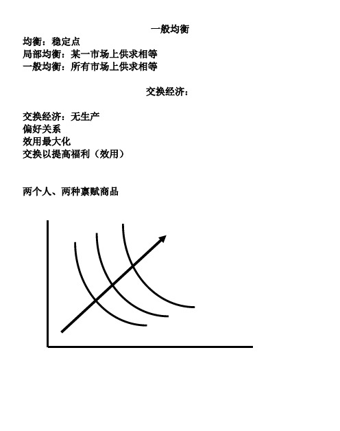
一般均衡均衡:稳定点局部均衡:某一市场上供求相等一般均衡:所有市场上供求相等交换经济:交换经济:无生产偏好关系效用最大化交换以提高福利(效用)两个人、两种禀赋商品Edgeworth 图 禀赋点为e假设自主交换能够实现帕累托改进,达到更优的配置点x对消费者1,其所偏好e 的区域为红色区域,最终的配置点必须在这一区域内,否那么,他拒绝交换或抵制这一配置。
对消费者2,其所偏好e 的区域为蓝色区域,最终的配置点必须在这一区域内,否那么,他拒绝交换或抵制这一配置。
因此,最终的配置点必须在重叠的区域中——凸透镜区域内和边上。
在这一区域里,双方或至少一方的福利能够提高。
11ee设交换后形成的配置点'x 在凸透镜内部,双方福利都得到改善,同时各有一条无差异曲线交于此点。
双方进一步通过交换改善彼此福利。
对消费者1,其所偏好'x 的区域为红色区域,最终的配置点必须在这一区域内,否那么,他拒绝交换或抵制这一配置。
对消费者2,其所偏好'x 的区域为蓝色区域,最终的配置点必须在这一区域内,否那么,他拒绝交换或抵制这一配置。
因此,最终的配置点必须在重叠的区域中——凸透镜区域内和边上。
在这一区域里,双方或至少一方的福利能够提高。
11ee'x交换过程持续下去,凸透镜越来越小,最终变为一个点:两条无差异曲线的切点:x 。
此时,双方进一步交换会使某一方福利下降。
所以,双方的交换一旦达到了切点位置,就不会有交换发生。
实现了帕累托最优。
在凸透镜内部和边上,这样的点有无数多个,最终的配置究竟是哪一个点,我们并不知道,或者说,我们不知道决定最终的帕累托效率点的位置的因素是什么。
结论只是:帕累托效率点位于凸透镜边上或内部的某个切点位置上。
11eexEdgeworth图中,所有的无差异曲线的切点的连线构成契约线,帕累托效率点是凸透镜与契约线交集中的点。
2 11eex当禀赋点落在契约线上时,即为帕累托效率点,无交换发生。
微观经济学Microeconomics-精品课件

• 参考教材 :黄亚钧 郁义鸿主编 《微观经 济学》,高等教育出版社,2003年。
• 参考书目: • [美]H.范里安著 《微观经济学:现代观
点》,上海三联书店 上海人民出版社, 1994年; • [美]平狄克 鲁宾费尔德 著 《微观经济 学》,中国人民大学出版社,1997年。 • 黎诣远 《微观经济分析》,清华大学出 版社
13、He who seize the right moment, is the right man.谁把握机遇,谁就心想事成。21.7.1421.7.1 401:18:2501:18 :25July 14, 2021
•
14、谁要是自己还没有发展培养和教 育好, 他就不 能发展 培养和 教育别 人。202 1年7月 14日星 期三上 午1时1 8分25 秒01:18:2521.nomic Man 经济人
• 如果说,稀缺是社会存在的经济概括, 那么,经济人这个概念就是对社会意 识的经济学概括。
• 经济学并不研究稀缺本身,而是研究 在稀缺条件下人的行为,也就是研究 经济人的行为。
© copyrights by Changde Zheng 2004. Economic college,Southwest University For Nationalities.
ii) Scarcity means that to have more of some things there must be less of others (Opportunity Cost): Production Possibilities Frontier
iii) Scarcity implies choice
•
15、一年之计,莫如树谷;十年之计 ,莫如 树木; 终身之 计,莫 如树人 。2021 年7月上 午1时1 8分21. 7.1401:18July 14, 2021
《微观经济学》PPT课件

〔2〕比较静态分析法:只分析 始点和终点的经济变量的 状 况
〔3〕动态分析法 引入时间因 素,分析某一时期内经济变量 的过程状况 .
三、经济模型
1、 经 济 模 型 〔economic
model>:用来表述经济
P price
变量之间的依存关系的理
李嘉图发展了亚当、斯密的思想,建立起了以劳动价 值论为基础,以分配论为中心的理论体系.并提出了 比较成本学说.他认为:每个国家都可以通过生产具 有相对优势的商品,通过国际贸易获得利益.
3、萨伊<Say>〔法〕 〔1767-1832〕
让·巴蒂斯特·萨伊
代表作《政治经济学概论》1803年
他认为:供给创造需求,储蓄必然转化 为投资,生产就是消费,供给就是需求, 生产过剩的危机是不会发生的.一个 国家生产者越多,产品越多,企业越多, 贸易越多社会财富越多.主张发展生 产.
2、按研究经济问题判断标准的不同可分为:
• 实证经济学<positive economics>:用事 实说明经济现象的现状如何?回答是什么 〔What is>如:某一时期的经济增长率为 8%,失业率是6%.
•规范经济学<normative economics>:以一 定的判断标准为出发点,力求回答应该是 什么〔What ought to be>.如:要实现8%的 年经济增长速度,政府应采取什么样的财 政政策和货币政策.某国的收入分配是不 是公平.
亚当、斯密的《国富论》
在《国富论》的序论中的第一句话就是: "被看作政治家或立法家的一门政治经济学 提出两个目标: 第一,给人民提供充足的收入或生计, 第二,给国家或社会提供充足的收入. 总之,其目的在于富国裕民".
高级微观经济学PPT课件

Slide 15
数学基础(一)
例1:在R1上的邻域
x0
B (x0 )
x 0 x0
B* (x0)
x0 x 0 x0
Slide 16
数学基础(一)
R 2上的邻域:
B (x0){xRn x-x0 }
x0
B (x 0)
x0
B * (x 0 )
Slide 17
数学基础(一)
开集S Rn
Slide 4
一个好模型
研究可观察的真实世界的各种现象,而不是虚构各种事实,或者研究虚拟世界 。解释的现象如果太特殊,理论没有意义,解释的现象如果太空泛,放之四海 的真理容易变成套套逻辑。
假设和“前提性假设”。假设为我们的研究设定了一个范围和条件,使待研究 的现象变得更简单,让研究者的精力集中在主要方面,而暂时忽略一些次要内 容。在满足这个假设条件下,得到的推论是可靠的。但是,关于假设条件是否 必须为真,经济学家之间通常有严重分歧。如弗里德曼认为,假设是否为真不 重要,重要的是得到的结论有比较普遍的解释能力。如理性假设、完全竞争市 场模型的四个假设条件、古诺模型的假设条件。
implies x z 。
Slide 13
数学基础(一)
度量与度量空间 欧氏空间
欧氏度量:x1, x2 n
d(x1,x2)(x1-x2)x (1-x2)
Slide 14
数学基础(一)
开邻域 B (x0 ), 0
B (x0){x R nd(x0,x)}
闭邻域
B
*
(
x
0
)
0
B*(x0){xnd(x0,x)}
一个好模型必须能够解释观察到的各种现象,推测的结果要用真实世界观察到 的现象或者素材来检验,一个好模型还必须是有可能被可证伪的。这样,理论 才能不断创新,不断发展。
高级微观经济课件

——愈来愈深化的问题,愈来愈能启发
新问题的问题。‛
5. 关于教材
教材:范里安:《微观经济学:现代观 点》(第八版),上海三联书店、上海人
民出版社2011年1月版
6. 主要参考书: 平狄克、鲁宾费尔德:《微观经济学》(
第七版),中国人民大学出版社2009年
7. 参考文献 ①图书:《经济学方法》,复旦大学出版社 2006年版 《青年经济学家指南》,上海财经大学出版 社2001年版 《应用经济学研究方法论》,经济科学出版 社1998年版 ②报刊杂志: 中国人民大学复印报刊资料经济类各专题、 CSSCI来源期刊
经济学中常用的数学理论
经济学是选择的科学,应用数学的目的——最优 化(优化理论) 数学分析、高等代数、微分方程、概率论、实变 函数、集合论、拓扑学、泛函分析——经济学语 言 经济学帝国主义——实证研究工具 社会科学研究现实的模式,数学研究逻辑可能的 模式。 理论研究:数理经济学(逻辑演绎) 经验研究:计量经济学(统计归纳)
数学(大海)与经济学(陆地)
人总希望脚踏实地。当被带离海岸线很远 时,会因失去对陆地的知觉而产生恐惧感 ,这是就初入海者而言的。渔民和航海家 则不同,他们会如鱼得水,如果把他们留 在岸边,他们会无所事事。但毕竟大多数 人都不是渔民和航海家,他们在海中游玩 时希望时刻看到岸边,并能随时上岸。岸 上的世界七彩斑斓,海中的世界单调乏味 ,但生命的本源却来自海洋。因此,我们 要培养自己在海中的生存能力。
know-what—知其然 显性知识 know-why—知其所以然 know-how—技巧、诀窍 隐性知识 know-who( 隔行如隔山
拥有:信息<知识<智慧<素质<觉悟
解决问题:?→。发现问题:?→? 波普尔《猜想与反驳》:‚科学和 知识的增长永远始于问题,终于问题
高级微观经济学2.ppt

analyze the maximum value function.
2008-09-10
18
2.1 Unconstrained Optimization
2008-09-10
19
2008-09-10
20
2008-09-10
21
2.2 Constrained Optimization
❖ 1. The same idea applies can be applied to the maximum-value function in constrained optimization.
2008-09-10
22
2008-09-10
23
2008-09-10
24
consume given income and prices.
❖ Note that the demand of a good depends on all prices. If we plot x1 (p, y) against pi, holding y and all prices other than pi constant, we get the demand curve of good i. A change in y or some pj , j≠ i, would be represented by a shift of the demand curve.
2008-09-10
4
2008-09-10
5
5. Proof:
❖ (a) Multiplying both prices and income by the same factor leaves the budget set unchanged.
《高级微观经济学》课件

考试安排
课程结束后将进行一次期末考试,考察学生对微观经济学理论和实践的理解和运用能力。
结语
通过学习高级微观经济学,您将拥有深入洞察经济问题的能力,成为经济学 的专家,并能运用所学知识解决实际经济问题。
研究消费者的偏好和选择行为,分析消费者 的需求曲线和边际效用。
市场结构和竞争
了解不同市场结构的特点,包括完全竞争、 垄断、寡头垄断和垄断竞争。
学习方法
1
课堂学习
通过听课和参与讨论,加深对微观经济学的理解和思考。
2
案例分析
通过分析实际经济问题和案例,将理论知识应用到实际情境中。
3
小组讨论
与同学一起合作讨论,分享思考和观点,促进深度学习和交流。
《高级微观经济学》 课件
让我们一起探索高级微观经济学的奥秘吧!本课程将帮助您深入了解微观经 济学的核心概念和分析方法,让您成为经济学的专家。
课程简介
通过本课程,您将了解微观经济学的基本原理和理论框架,掌握市场经济中个体和企业的行为分析方法, 以及了解市场失灵和政府干预等相关问题。
教材介绍
我们将使用《高级微观经济学》教材,该教材包含了丰富的案例研究和实际 问题分析,帮助学生将理论知识应用到实际经济问题中。
课程目标
本课程的目标是帮助学生深入理解微观经济学的核心概念,掌握经济学的思维方式和分析工具,以及培 养学生独立思考和问题解决的能力。
主要内容
供求关系分析
通过供求关系曲线的分析,了解市场价格和 数量的决定因素。
生产者行为分析
研究生产者的成本和利润最大化行为,分析 生产者的供给曲线和边际成本。
消费者行为分析
高级微观经济学(清华大学-武康平)ppt课件

.
7
特点之二:逻辑思辨
从方法论上讲,高级经济学是数学思辨模式的
经济学,数学构成了她的方法论基础。
高级经济学力图使经济学成为真正的科学。这
样一来,她就离不开逻辑分析工具的运用。她对经
济问题的研究,总是从一系列假设前提出发,来建
立起经济现象的理论模型,并经过严密的逻辑推理
分析,得出结论,然后又应用理论去指导实践。
的来设计的。
具体包括:微观经济学发展动态、消费者行为
理论、需求理论、不确定条件下的选择、理性生产
者行为分析、竞争与垄断、博弈论、一般均衡与社
会福利。
这些内容可以帮助学员进一步提高分析、解决
经济问题的能力,建立起经济学的思维方式,加深
对经济学的理解。但因课时限制,其中的部分内容
要求学员根据教材《高级微. 观经济学》自学。
高级微观经济学
课程简介
任课教师:武康平
2008年9月15日
.
1
课程教材 高级微观经济学
武康平 编著 清华大学出版社,2001年版
参考书
Microeconomic Theory
by A. Mas-Colell, M. D. Whinston & J. R. Green,
Oxford University.Press(1995)
dijg.06@
.
3
课程讨论区
学院主页课程讨论区高级微观经济学
序 号:
学生帐号: 学生口令:
助教帐号: 助教口令:
.
4
I. 经济学的学习层次
西方经济学一般要分为三个层次来逐步学习: 初级 中级 高级
初级:本科一年级,启蒙阶段,经济学入门课程,目的是帮 助学员建立起经济学的直观概念。
高级微观经济学 (黄有光) Advanced Microeconomics-Topic 3-Consumer
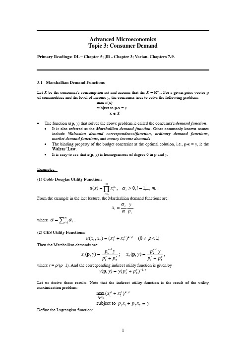
Advanced Microeconomics Topic 3: Consumer DemandPrimary Readings: DL – Chapter 5; JR - Chapter 3; Varian, Chapters 7-9.3.1 Marshallian Demand FunctionsLet X be the consumer's consumption set and assume that the X = R m +. For a given price vector p of commodities and the level of income y , the consumer tries to solve the following problem:max u (x )subject to p ⋅x = y x ∈ X• The function x (p , y ) that solves the above problem is called the consumer's demand function .• It is also referred as the Marshallian demand function . Other commonly known namesinclude Walrasian demand correspondence/function , ordinary demand functions , market demand functions , and money income demands .• The binding property of the budget constraint at the optimal solution, i.e., p ⋅x = y , is theWalras’ Law .• It is easy to see that x (p , y ) is homogeneous of degree 0 in p and y .Examples:(1) Cobb-Douglas Utility Function:.,...,1,0 ,)(1m i x x u i mi i i =>=∏=ααFrom the example in the last lecture, the Marshallian demand functions are:.ii i p yx αα=where∑==mi i 1αα.(2) CES Utility Functions: )10( )(),(/12121<≠+=ρρρρx x x x uThen the Marshallian demands are:,),( ;),(2112221111rr r r r r p p yp y x p p y p y x +=+=--p p where r = ρ/(ρ -1). And the corresponding indirect utility function is given byrr r p p y y v /121)(),(-+=pLet us derive these results. Note that the indirect utility function is the result of the utility maximization problem:yx p x p x x x x =++2211/121, subject to )(max 21ρρρDefine the Lagrangian function:)()(),,(2211/12121y x p x p x x x x L -+-+=λλρρρThe FOCs are:00)(0)(22112121)/1(2121111)/1(211=-+=∂∂=-+=∂∂=-+=∂∂----y x p x p Lp x x x x L p x x x x L λλλρρρρρρρρ Eliminating λ, we get⎪⎩⎪⎨⎧+=⎪⎪⎭⎫⎝⎛=-2211)1/(12121x p x p y p p x x ρ So the Marshallian demand functions are:rr r rrr p p yp y x x p p yp y x x 211222211111),(),(+==+==--p pwith r = ρ/(ρ-1). So the corresponding indirect utility function is given by:r r r p p y y x y x u y v /12121)()),(),,((),(-+==p p p3.2 Optimality Conditions for Co nsumer’s ProblemFirst-Order ConditionsThe Lagrangian for the utility maximization problem can be written asL = u (x ) - λ( p ⋅x - y ).Then the first-order conditions for an interior solution are:yu i p x u i i =⋅=∇∀=∂∂x p p x x λλ)( i.e. ;)( (1)Rewriting the first set of conditions in (1) leads to,,k j p p MU MU MRS kj kj kj ≠==which is a direct generalization of the tangency condition for two-commodity case.Sufficiency of First-Order ConditionsProposition : Suppose that u (x ) is continuous and quasiconcave on R m +, and that (p , y ) > 0. If u if differentiable at x*, and (x*, λ*) > 0 solves (1), then x* solve the consumer's utility maximization problem at prices p and income y .Proof . We will use the following fact without a proof:• For all x , x ' ≥ 0 such that u (x') ≥ u (x ), if u is quasiconcave and differentiable at x , then∇u (x )(x' - x ) ≥ 0.Now suppose that ∇u (x*) exists and (x*, λ*) > 0 solves (1). Then,∇u (x*) = λ*p , p ⋅x* = y .If x* is not utility-maximizing, then must exist some x 0 ≥ 0 such thatu (x 0) > u (x*) and p ⋅x 0 ≤ y .Since u is continuous and y > 0, the above inequalities implies thatu (t x 0) > u (x*) and p ⋅(t x 0) < yfor some t ∈ [0, 1] close enough to one. Letting x' = t x 0, we then have∇u (x*)(x' - x ) = (λ*p )⋅( x' - x ) = λ*( p ⋅x' - p ⋅x ) < λ*(y - y ) = 0,which contradicts to the fact presented at the beginning of the proof since u (x 1) > u (x*).Remark• Note that the requirement that (x*, λ*) > 0 means that the result is true only forinterior solutions.Roy's IdentityNote that the indirect utility function is defined as the "value function" of the utility maximization problem. Therefore, we can use the Envelope Theorem to quickly derive the famous Roy's identity.Proposition (Roy's Identity?): If the indirect utility function v (p , y ) is differentiable at (p 0, y 0) and assume that ∂v (p 0, y 0)/ ∂y ≠ 0, then.,...,1 ,),(),(),(000000m i yy v p y v y x ii =∂∂∂∂-=p p pProof . Let x * = x (p , y ) and λ* be the optimal solution associated with the Lagrangian function:L = u (x ) - λ( p ⋅x - y ).First applying the Envelope Theorem, to evaluate ∂v (p 0, y 0)/ ∂p i gives.**)*,(),(*i ii x p L p y v λλ-=∂∂=∂∂x p But it is clear that λ* = ∂v (p , y )/ ∂y , which immediately leads to the Roy's identity.Exercise• Verify the Roy's identity for CES utility function.Inverse Demand FunctionsSometimes, it is convenient to express price vector in terms of the quantity demanded, which leads to the so-called inverse demand functions .• the inverse demand function may not always exist. But the following conditions willguarantee the existence of p (x ):• u is continuous, strictly monotonic and strictly quasiconcave. (In fact, these conditionswill imply that the Marshallian demand functions are uniquely defined.)Exercise (Duality of Indirect and Direct Demand Functions):(1) Show that for y = 1 the inverse demand function p = p (x ) is given by:.,...,1 ,)()()(1m i x x u x u p m j j jii =∂∂∂∂=∑=x x x(Consult JR, pp.79-80.)(2) Show that for y = 1, the (direct) demand function x = x (p, 1) satisfies.,...,1 ,)1,()1,()1,(1m i p p v p v x m j j j ii =∂∂∂∂=∑=p p p(Hint: Use Roy’s identity and the homogeneity of degree zero of the indirect uti lityfunction.)3.3 Hicksian Demand FunctionsRecall that the expenditure function e (p , u ) is the minimum-value function of the following optimization problem:,)( s.t. min ),(u u u e m≥⋅=+∈x x p p R x for all p > 0 and all attainable utility levels.It is clear that e (p , u ) is well-defined because for p ∈ R m ++, x ∈ R m +, p ⋅x ≥ 0.If the utility function u is continuous and strictly quasiconcave, then the solution to the above problem is unique, so we can denote the solution as the function x h (p , u ) ≥ 0. By definition, it follows thate (p , u ) = p ⋅x h (p , u ).• x h (p , u ) is called the compensated demand functions , also commonly known as Hicksiandemand functions , named after John Hicks when he first discussed this type of demand functions in 1939.Remarks1. The reason that they are called "compensated " demand function is that we mustimpose an artificial income adjustment when the price of one good is changing while the utility level is assumed to be fixed.2. It is important to understand that, in contrast with the Marshallian demands, theHicksian demands are not directly observable.As usual, it should be no longer a surprise that there is a close link between the expenditure function and the Hicksian demands, as summarized in the following result, which is again a direct application of the Envelope Theorem..Proposition (Shephard's Lemma for Consumer): If e (p , u ) is differentiable in p at (p 0, u 0) with p 0 > 0, then,.,...,1 ,),(),(000m i p u e u x ih i=∂∂=p pExample: CES Utility Functions)10( )(),(/12121<≠+=ρρρρx x x x uLet us now derive the Hicksian demands and the corresponding expenditure function.min {p 1x 1 + p 2x 2} subject to)(/121u x x =+ρρρThe Lagrangian function is))((),,(/121221121u x x x p x p x x L -+-+=ρρρλλThen the FOCs are:0)(0)((0)((/121121/12122111/12111=+-=∂∂=+-=∂∂=+-=∂∂----ρρρρρρρρρρρλλλx x u L x x x p x L x x x p x L Eliminating λ, we getρρρρ/121)1/(12121)(x x u p p x x +=⎪⎪⎭⎫ ⎝⎛=- From these, it is easy to derive the Hicksian demand functions given by:121)/1(212111)/1(211)(),()(),(----+=+=r r r r h r r r r h pp p u u x p p p u u x p pwhere r = ρ/(ρ-1). And the expenditure function is.)(),(),(),(/1212211rr r h h p p u u x p u x p u e +=+=p p pAlternatively, since we know that the indirect utility function is given by:,)(),(/121rr r p p y y v -+=p3.4 Recall that (last the indirect utility function v (p (a) e (p , v (b) v (p , eFurthermore, we solutions ofboth optimization the following interesting identities between Marshallian demands and Hicksian demands:x (p , y ) = x h (p , v (p , y )) x h (p , u ) = x (p , e (p , u ))which hold for all values of p , y and u .The second identity leads to a classic differentiation relation between Hicksian demands and Marshallian demands, known as Slutsky equation.Proposition (Slutsky Equation): If the Marshallian and Hicksian demands are all well-defined and continuously differentiable, then for p > 0, x > 0,),,(),(),(),(y x yy x p u x p y x j i j h i j i p p p p ⋅∂∂-∂∂=∂∂where u = v (p , y ).Proof . It follows easily from taking derivative and applying Shephard's Lemma.Substitution and Income Effects• The significance of Slutsky equation is that it decomposes the change caused by a pricechange into two effects: a substitution effect and an income effect .• The substitution effect is the change in compensated demand due to the change inrelative prices, which is the first item in Slutsky equation.• The income effect is the change in demand due to the effective change in incomecaused by the price change, which is the second item in Slutsky equation. • The substitution effect is unobservable, while the income effect is observable.Question: From the above diagram (also know as Hicksian decomposition ), can you see crossing property between a Marshallian demand function and the corresponding Hicksian demand? (Hint: there are two general cases.)Slutsky MatrixThe substitution effect between good i and good j is measured byj i p u x s jh i ij ,,),(∀∂∂=pSo the Slutsky matrix or the substitution matrix is the m ⨯m matrix of the substitution items:⎥⎥⎦⎤⎢⎢⎣⎡∂∂==j h i ij p u x s ),(][p SThe following result summarizes the basic properties of the Slutsky matrix.Proposition (Substitution Properties). The Slutsky matrix S is symmetric and negative semidefinite.Proof . By Shephard’s Lemma (for consumer), we know thatji ihj i j j i j h i ij s p u x p p u e p p u e p u x s =∂∂=∂∂∂=∂∂∂=∂∂=),(),(),(),(22p p p pHence S is symmetric. It is evident that S is the Hessian matrix of the expenditure function e (p , u ).Since we know that e (p , u ) is concave, so its Hessian matrix must be negative semidefinite.Since the second-order own partial derivatives of a concave function are always nonpositive, this implies that s ii ≤ 0, i.e.,i p u x s ih i ii ∀≤∂∂=,0),(pwhich indicates the intuitive property of a demand function: as its own price increases, the quantity demanded will decrease. You are reminded that this is a general property for Hicksian demands.For the Marshallian demands, note that by Slutsky equation,).,(),(),(),(y x yy x p u x p y x i i i h i i i p p p p ⋅∂∂-∂∂=∂∂Then for a small change in p i , we will have the following:.),(),(),(),(i i i i i h i i i i i p y x yy x p p u x p p y x x ∆⋅∂∂-∆∂∂=∆∂∂≈∆p p p pThe first item, capturing the own price effect of the Hicksian demands, is of course nonpositive.The sign of the second item depends on the nature of the good:• Normal good : ∂x i (p , y )/ ∂y > 0.• This leads to a normal Marshallian demand function: it is decreasing in its ownprice.• Inferior good : ∂x i (p , y )/ ∂y < 0.• When the substitution effect still dominates the income effect, the resultingMarshallian demand is also decreasing in its own price.• When the substitution effect is dominated by the income effect, it will lead to aGiffen good, that is, its demand function is an increasing function of its own price.Because of Slutsky equation, the Slutsky matrix (i.e., the substitution matrix) also has the following form that is in terms of Marshallian demand functions.⎥⎥⎦⎤⎢⎢⎣⎡∂∂+∂∂=⎥⎥⎦⎤⎢⎢⎣⎡∂∂==),(),(),(),(][y x y y x p y x p u x s j i j i j h i ij p p p p SWe will get back to the above Slutsky matrix in the next lecture when we discuss the integrability problem .3.5. The Elasticity Relations for Marshallian Demand FunctionsDefinition . Let x (p , y ) be the consumer’s Marshallian demand functions. Define.),(,),(),(,),(),(yy x p s y x p p y x y x yy y x i i i i jj i ij i i i p p p p p =∂∂=∂∂=εηThen1. ηi is called the income elasticity of demand for good i .2. ε ij is called the price elasticity of the demand for good i with respect to a price change ingood j . ε ii is the own-price elasticity of the demand for good i . For i ≠ j , ε ij is the cross-price elasticity .3. s i is called the income share spent on good i .The following result summarizes some important relationships among the income shares, income elasticities and the price elasticities.Proposition . Let x (p , y ) be the consumer’s Marshallian demand functions. Then1. Engel aggregation :.11=∑=mi ii s η2. Cournot aggregation :.,...,1 ,1m j s s j mi iji =-=∑=εProof . Both identities are derived from the Walras’ Law, namely, the fact that the budget is tight or balanced:y = p ⋅x (p , y ) for all p and y . (A)To prove Engel aggregation, we differentiate both sides of (A) w.r.t. y :∑∑∑====∂∂=∂∂=m i mi i i ii i i mi i i s y x yy y x y y x p y y x p 111,),(),(),(),(1ηp p p pas required.To prove Cournot aggregation, we differentiate both sides of (A) w.r.t. p j :.),(),(),(),(),(01∑∑=≠∂∂=-⇒∂∂++∂∂=mi j i i j jj jj ji j i ip y x p y x p y x p y x p y x p p p p p pMultiplying both sides by p j /y leads to∑∑∑====-⇒∂∂=∂∂=-mi iji j mi i jj i i i mi j j i i j j s s y x p p y x y y x p p p y x y p yy x p 111),(),(),(),(),(εp p p p pas required too.3.6 Hicks ’ Composite Commodity TheoremAny group of goods & services with no change in relative prices between themselves may be treated as a single composite commodity, with the price of any one of the group used as the price of the composite good and the quantity of the composite good defined as the aggregate value of the whole group divided by this price. Important use in applied economic analysis.Additional ReferencesAfriat, S. (1967) "The Construction of Utility Functions from Expenditure Data," International Economic Review, 8, 67-77.Arrow, K. J. (1951, 1963) Social Choice and Individual Values. 1st Ed., Yale University Press, New Haven, 1951; 2nd Ed., John Wiley & Sons, New York, 1963.Becker, G. S. (1962) "Irrational Behavior and Economic Theory," Journal of Political Economy, 70, 1-13.Cook, P. (1972) "A One-line Proof of the Slutsky Equation," American Economic Review, 42, 139. Deaton, A. and J. Muellbauer (1980) Economics and Consumer Behavior. Cambridge University Press, Cambridge.Debreu, G. (1959) Theory of Value. John Wiley & Sons, New York.Debreu, G. (1960) "Topological Methods in Cardinal Utility Theory," in Mathematical Methods in the Social Sciences, ed. K. J. Arrow and M. D. Intriligator, North Holland, Amsterdam. Diewert, W. E. (1982) "Duality Approaches to Microeconomic Theory," Chapter 12 in Handbook of Mathematical Economics, ed. K. J. Arrow and M. D. Intriligator, North Holland, Amsterdam.Gorman, T. (1953) “Community Preference Fields,” Econometrica, 21, 63-80.Hicks, J. (1946) V alue and Capital. Clarendon Press, Oxford, England.Katzner, D.W. (1970) Static Demand Theory. MacMillan, New York.Marshall, A. (1920) Principle of Economics, 8th Ed. MacMillan, London.McKenzie, L. (1957) “Demand Theory Without a Utility In dex," Review of Economic Studies, 24, 183-189.Pollak, R. (1969) "Conditional Demand Functions and Consumption Theory," Quarterly Journal of Economics, 83, 60-78.Roy, R. (1942) De l'utilite. Hermann, Paris.Roy, R. (1947) "La distribution de revenu entre les divers biens," Econometrica, 15, 205-225. Samuelson, P. A. (1938) "A Note on the Pure Theory of Consumer's Behavior," Econometrica, 5, 61-71, 353-354.Samuelson, P. (1947) Foundations of Economic Analysis. Harvard University Press, Cambridge, Massachusetts.Sen, (1970) Collective Choice and Social Welfare. Holden Day, San Francisco.Stigler, G. (1950) "Development of Utility Theory," Journal of Political Economy, 59, parts 1 & 2, pp. 307-327, 373-396.Varian, H. R. (1992) Microeconomic Analysis. Third Edition. W.W. Norton & Company, New York. (Chapters 7, 8 and 9)Wold, H. and L. Jureen (1953) Demand Analysis. John Wiley & Sons, New York.11。
上财高级微观范翠红科课件一

Cuihong Fan
Chapter 1 Consumer Theory
15/21
Definition (2)
The preference relation on X is continuous if for all x ∈ X , the upper contour set {y ∈ X : y x } and the lower contour set y ∈ X : x y are both closed in X .
Cuihong Fan
Chapter 1 Consumer Theory
16/21
II. Utility function
1. Definition
Definition (Utility function)
A real-valued function u : X → R is called a utility function representing the preference if for any consumption bundles x, y ∈ X , x y ⇐⇒ u (x ) ≥ u (y ).
y if either x1 > y1 or
Example
1 Consider the sequences of bundles x n = ( n , 0) and y n = (0, 1), show that the lexicographic preferences are not continuous.
Not all rational preferences are continuous
Cuihong Fan
Chapter 1 Consumer Theory
《高级微观经济学》课件

公共支出
政府通过提供公共服务和基础 设施,弥补市场失灵,提高社 会福利。
监管和行政干预
政府对市场进行监管和行政干 预,防止垄断和不公平竞争。
市场失灵与政府干预的案例分析
环境污染案例
政府通过制定环保法规和排污标准,限制企 业排污,保护环境。
医疗保障案例
政府通过提供医疗保险和医疗救助,弥补市 场失灵,保障公民健康。
最优消费选择
在预算约束下,消费者选择能够最大化效用的商品组合。
边际替代效应
描述消费者在保持效用不变的情况下,一种商品对另一种商品的 替代程度。
消费者行为理论的扩展
风险偏好与不确定性
研究消费者在面临风险和不确定性时的消费行 为。
跨期消费选择
探讨消费者在不同时期之间的消费决策和储蓄 行为。
消费外部性
分析消费行为对其他个体或社会的影响,以及如何通过政策干预来改善消费行 为。
微观经济学的重要性
微观经济学是现代经济学的重要组成部分,它为政策制定者、企业家和消费者提供了理解和预测市场运作的基础 。通过研究微观经济学,人们可以更好地理解市场机制、价格体系和资源配置,从而做出更明智的决策。
微观经济学的基本假设和概念
基本假设
微观经济学通常基于一些基本假设, 如完全竞争、理性行为、完全信息等 。这些假设为理论分析提供了基础, 但在实际生活中可能并不完全成立。
公共选择理论与政治经济学
01
公共选择理论
研究公共物品和服务的供给和需求,以及政府决策的经济学分析。
02
政治经济学
研究政治和经济之间的相互作用,以及政治制度对经济发展的影响。
03
总结
公共选择理论和政治经济学是微观经济学的前沿领域,它们对于理解政
《微观经济学microeconomics》英文版全套课件(101页)

The economic constraint:
px p1x1 ... pL xL w
The Walrasian budget set (Definition 2.D.1)
Bp,w {x RL : px w}
or
u(x* ) xl
pl
px w
Solution: Walrasian demand function x*( p, w)
Utility Maximization -- Example
Example 3.D.1: the transformed Cobb-Douglas Utility Function
Expenditure Function
Expenditure function e( p,u) Min px s.t. u(x) u {x}
Properties: 1. Homogeneous of degree of one in p 2. Strictly increasing in u and nondecreasing in p 3. Concave in p 4. Continuous in p and u
Comparative Statics – Wealth Effects
The consumer’s Engel function x( p, w)
The wealth effect xl ( p, w) / w or Dwx( p, w) Normal goods and inferior goods
A choice rule C(B) B
The weak axiom of revealed preference (WARP): if x is revealed at least as good as y, then y cannot be revealed preferred to x
高级微观经济学讲义-577页文档

(PF = 1/2)
(PF = 2)
食物
40
80
120
Chapter 1
160 (单位/周)
28
预算约束
预算约束
• 两件商品和劳务
P X X P Y Y I,X 0 ,Y 0
• N件商品和劳务
P 1 X 1 P 2 X 2 P n X n I ,X i 0 , i 1 , 2 , n
O
50
C
Chapter 1
33
消费者偏好和无差异曲线
关于消费选择的基本假设
• 完备性假设:给定消费空间里任何一对消费组 合A和B,下列三者关系之一必成立:或者A>B, 或者B>A,或者A∽B。这意味着,消费者可以 在两组消费组合中作出一种明确的判断。
Chapter 1
34
消费者偏好和无差异曲线
预期、相关商品的价格 • 需求函数(求曲线) • 需求的变动和需求量的变动 • 需求规律(法则)
Chapter 1
15
经济学基础-需求和供给
供给
• 企业供给、市场供给 • 价格、生产技术、劳动、资本、原料等的投入
品价格 • 供给函数(供给曲线) • 供给的变动和供给量的变动 • 供给规律(法则)
Chapter 1
36
消费者偏好和无差异曲线
无差异曲线
无差异曲线代表了能给一个人相同程度满足 的市场篮子的所有商品组合。
无差异曲线包含了全体给予某消费者同等满 意程度的消费组合。
Chapter 1
37
消费者偏好和无差异曲线
衣服(单位/周)
50
B
40
H
比起蓝色方框中的任一市场篮子, 消费者偏好于市场篮子A; 而比起市场篮子A,消费者偏好于 粉红色方框中的任一市场篮子。 (“多比少好”的第三个假定)
瓦里安高级微观经济学--技术PPT课件

14
4. 规模报酬(Return to Scale)
也称为规模经济,描述要素投入和产出量之间的 关系,或者投入导致产出量变化的关系。
规模与收益变化的可行集
产出的可行集特征:产出的可扩张性。即 对于任意t 0,如果y Y ,则有ty Y
投入的可行集特征:投入可扩张性。即 对于任意t 0,如果x V ( y),则有tx V (ty)
T : n
Y {y n :T(y) 0}
当且仅当 y 是技术有效时,那么:
T(y) 0
Y {y n :T (y) 0}
y1
6
生产函数及其描述
生产函数的一般形式
f ( X ) max{ y ( y, x1, x2 ,, xn ) Y}
生产可能集的描述
等产量线:
Q(y) {(x1, x2 ) R2 : y x1 x21- }
转化函数
T(y) {y y - x1 x12- 0}
8
2. 技术(生产可能集)的特征
正则性(Regular technology)
对于所有的产出y≥0,要素需求集V(y)是非
空的
任何给定的产出水平都是可以通过一定数量的投 入来实现的
要素需求集V(y) 是闭集
要素需求集包括它自己的边界
厂商不可能在没有投入的情况下生产出某种
产出(No free lunch)
——规范性?
9
单调性(Monotonity)
要素需求集的单调性
如果x在V(y)中,并且x′≥x,那么x′也在V(y)
中。 意义为投入增加产出不会降低。 要素需求集的单调性隐含着要素的可自由处
微观经济学高级版英文原版课件
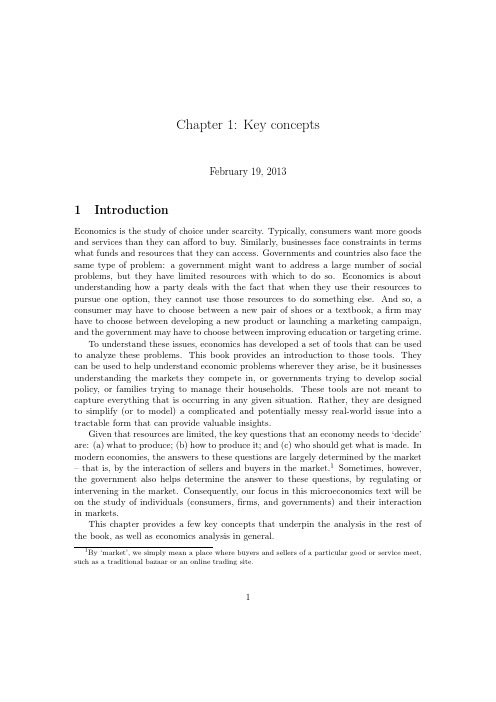
Chapter1:Key conceptsFebruary19,20131IntroductionEconomics is the study of choice under scarcity.Typically,consumers want more goods and services than they can afford to buy.Similarly,businesses face constraints in terms what funds and resources that they can ernments and countries also face the same type of problem:a government might want to address a large number of social problems,but they have limited resources with which to do so.Economics is about understanding how a party deals with the fact that when they use their resources to pursue one option,they cannot use those resources to do something else.And so,a consumer may have to choose between a new pair of shoes or a textbook,afirm may have to choose between developing a new product or launching a marketing campaign, and the government may have to choose between improving education or targeting crime.To understand these issues,economics has developed a set of tools that can be used to analyze these problems.This book provides an introduction to those tools.They can be used to help understand economic problems wherever they arise,be it businesses understanding the markets they compete in,or governments trying to develop social policy,or families trying to manage their households.These tools are not meant to capture everything that is occurring in any given situation.Rather,they are designed to simplify(or to model)a complicated and potentially messy real-world issue into a tractable form that can provide valuable insights.Given that resources are limited,the key questions that an economy needs to‘decide’are:(a)what to produce;(b)how to produce it;and(c)who should get what is made.In modern economies,the answers to these questions are largely determined by the market –that is,by the interaction of sellers and buyers in the market.1Sometimes,however, the government also helps determine the answer to these questions,by regulating or intervening in the market.Consequently,our focus in this microeconomics text will be on the study of individuals(consumers,firms,and governments)and their interaction in markets.This chapter provides a few key concepts that underpin the analysis in the rest of the book,as well as economics analysis in general.1By‘market’,we simply mean a place where buyers and sellers of a particular good or service meet, such as a traditional bazaar or an online trading site.12Scarcity and opportunity costAs noted above,it is usually the case that resources are limited,so that not all wants can be met.We call this situation scarcity.Scarcity also means that individuals,businesses and societies face tradeoffs;by choos-ing one thing,a person must give up or miss out on another thing.For example,if a consumer uses their money to buy product X,they cannot then use that same money to buy something else.2We use the concept of opportunity cost to measure that tradeoff. Thus,the opportunity cost of any choice is the value of the best forgone alternative. In the example above,if the consumer buys product X,and the next best thing they could have done is buy product Y,the opportunity cost of buying X is forgoing Y.Individuals also face opportunity costs in terms of their time–that is,if a person spends his time doing one thing,he cannot also spend that time doing another.Example.Suppose Andrew prefers to spend his Saturday afternoon walk-ing.The next best thing that he could have done is to sleep,and his thirdbest choice is to go swimming.Therefore,if Andrew goes for a walk,the op-portunity cost of going for a walk is not sleeping,as this is his best foregoneopportunity.The option of swimming is not relevant here because it is notthe next best opportunity.Opportunity costs include both explicit costs and implicit costs.Explicit costs are costs that involve direct payment(or,in other words,would be considered as costs by an accountant).Implicit costs are opportunities that are forgone,but do not involve an explicit cost.3Example.Suppose Stephen decides to go to university,and his next bestoption is to work at a construction site and earn$80K over the year.Theexplicit costs are those that Stephen must directly pay to go to university,such as student fees,the cost of textbooks,and so on.The implicit costsare the opportunities that Stephen must forgo–that is,working at theconstruction site and earning$80K.It is important to note that opportunity cost only includes costs that could change if a different decision were made.Opportunity cost does not include sunk(or unrecoverable) costs.Sunk costs are costs that have been incurred and cannot be recovered no matter what.For example,if Katrien spends the weekend reading an accounting textbook, no matter what she does(such as whether or not she decides to continue studying accounting),she cannot get that time back.Similarly,if a business spent$100K on an advertising campaign last year,regardless of what they decide to do this year,that money(and effort)cannot be recovered.2It is common to hear people refer to the‘economics’of a particular thing.This colloquial statement really means that,given the limited resource available,a choice had to be made and something(possibly worthwhile)could not be done.3Sometimes,economists distinguish between‘economic costs’and‘accounting costs’.Economic costs is just another term for opportunity costs,and therefore includes explicit and implicit costs. Accounting costs refers to explicit costs only.23Marginal analysisTypically,we assume that economic agents are rational and act to maximize their benefits from their economic transactions.4For example,consumers seek to maximize their benefits from consumption andfirms seek to maximize their profits from production. One way that economic agents can solve this maximization problem is by considering the additional benefit or additional cost of any action.This sort of analysis is referred to as marginal analysis and it is a recurring theme both in this book and economics generally.For instance,consider a consumer faced with the decision of whether to buy one more unit of a particular good.That consumer might consider the extra benefit he derives from buying that extra unit;this is referred to as the marginal benefit of that extra unit of the good.The consumer might also consider the additional cost of buying one more unit;this is referred to as the marginal cost of purchasing another unit,which is typically the price of the good.In making theirfinal decision,the consumer will weigh the marginal benefit against the marginal cost of buying that extra unit.For example, if a consumer is considering buying another cup of coffee,and the marginal benefit is$5 and the marginal cost is$3,the consumer will be better offby buying the extra coffee.Each of the marginal terms noted above,and many others,will be discussed at length throughout the book.What is crucial to note is that the term‘marginal’simply means means additional or extra.That is,we interested to see what happens if we increase things(such as the number of coffees bought)by a small amount.4Ceteris paribusThe notion of ceteris paribus is also an important foundation of economic analysis.As noted,because the real world is often complicated and messy,it is often necessary to simplify real-world situations into tractable economic models,in order to better analyze them.Thus,in order to determine the effect of a particular thing,economists tend to examine the impact of one change at a time,holding everything else constant.This is often called ceteris paribus,which roughly means‘other things equal’.For instance,suppose we are interested in how a change in price will affect the quantity demanded of a good.However,in reality,demand for a good can be affected by a number of other factors,such as changes in the tastes or income of consumers,or the availability or price of substitute goods.Therefore,in order to isolate the effect of price upon quantity demanded,we need hold everything else constant.This is not to deny that in the real world multiple changes can occur at a time–they often do.Rather, to fully understand the relationship between price and demand,it is essential to isolate that relationship from other events that might also be occurring.For example,afirm 4We are not suggesting that,in the real word,consumers are always fully rational or thatfirms do not sometimes have other objectives.Rather,we adopt this simplifying assumption because it allows us to analyze the behaviour of economic agents in markets.Such analysis will be fairly accurate,provided that on average individual consumers andfirms act more or less in their own interest.3might be interested in the effect of advertising on demand for its product.To understand the impact of advertising,it is crucial to remove other factors that could affect demand, otherwise advertising could be attributed too much(or too little)influence,which could lead to poor decision-making by thefirm regarding its next advertising campaign.5Correlation and causationAnother factor to keep in mind is the difference between correlation and causation. Correlation refers to a situation in which two or more things are observed to move together(or against each other).On the other hand,causation refers to a situation where changes in one thing brings about or causes change in another thing.To make statements about causation requires an economic theory about how the world works, rather than just observing a statistical relationship between several variables.Sometimes,when we observe correlation between two variables,A and B,it is because one causes the other.Sometimes,it is because a third factor causes changes in A and B(like a rising tide causing two boats to rise in their moorings).Sometimes,there is no connection between the two variables and it is just by chance that we observed the change in both variables at the same time.Without a theory about how a change in one variable affects the other,it is not possible to say which is the case.4。
- 1、下载文档前请自行甄别文档内容的完整性,平台不提供额外的编辑、内容补充、找答案等附加服务。
- 2、"仅部分预览"的文档,不可在线预览部分如存在完整性等问题,可反馈申请退款(可完整预览的文档不适用该条件!)。
- 3、如文档侵犯您的权益,请联系客服反馈,我们会尽快为您处理(人工客服工作时间:9:00-18:30)。
2.Properties of PS.
• Additive (free entrance) :
y Y,and y Y, then y y Y • Convexity: y Y,and y Y, then y (1 )y Y, here [0,1]
See the fig.
• Proposition1: if Y is convex, so is V(q). • Proposition2: if V(q) is convex, f(x) is quasiconcave.
lecture 1 for Chu Kechen Honors College
y Y, ay Y, a 0
lecture 1 for Chu Kechen Honors College
4.Returns to scale
• Proposition 3: Y is constant returns to
scale if Y is both “additive” and “convexity”. • Proposition 4: single production, if and only if f(.) is homogenous of degree 1, Y is constant returns to scale.
the array y y, and y Y means y Y • No free lunch: Y n {0}
n n
See the fig.
• Free disposal:
See the fig.
lecture 1
y n Y
for Chu Kechen Honors College
xj xi
• Question2: calculate the “TRS” and the
“elasticity of substitution” of CobbDouglas technology and CES technology.
for Chu Kechen Honors College
lecture 1
– Homothetic function:
for Chu Kechen Honors College
lecture 1
Assignment
• Textbook: ex.1.1, ex.1.3, ex.1.7. ex.1.9
lecture 1
for Chu Kechen Honors College
– Some of yi in y are restricted on z . – Short-run production set.
lecture 1
for Chu Kechen Honors College
1. Production set
• Input requirement set:
– All yi in y are negative, let them be –x (then x is positive), and the rest yj to be q . I O n – So, x and q , and y (q,-x) – the input requirement set is :
lecture 1 for Chu Kechen Honors College
4.Returns to scale
• Homogeneous and homothetic tech.
– Homogeneous of degree k:
f (tx) t k f (x) t 0
•
f (x) g (h(x)) h(x) is HD1, g (.) is a possitive monotonic function. Elasticity of scale: d ln q(t ) e( x ) q(t ) f (tx) d ln t t 1
lecture 1 for Chu Kechen Honors College
– If O = 1,and I = n - 1, then:
2.Properties of PS.
• Y is nonempty: we have something to do. • Y is close: Y contain it’s boundary,
y2
T ( y )
{ y : T ( y) 0}
y1
MRT12
{ y : T ( y) 0}
lecture 1
for Chu Kechen Honors College
lecture 1
for Chu Kechen Honors College
lecture 1
for Chu Kechen Honors College
1. Production set
• Production plan (production vector, or
input-output vector): y ( y1 , y2 , , yn ) • Production set Y: all technological feasible y. Y {y n : y are technologically feasible} • Restricted production set Y (z):
Choice
(purchase)
Choice
lecture 1
for Chu Kechen Honors College
Technology
• Contain:
– “production (possibilities) set” (PS) and “production function”; – Properties of the “PS”; – Technical rate of substitution; – Returns to scale.
4.Returns to scale
• Nonincreasing returns to scale:
y Y, ay Y, a [0,1] y Y, ay Y, a 1
• Nondecreasing returns to scale:
• Constant return to scale:
Advanced Microeconomics
(lecture 1: production theory I)
Summary
• textbook: • assignments:
– Varian, Hal R., 1992, Microeconomics Analysis, 3rd ed. – Mas-Colell, A., M. Whinston, and J. Green, 1995, Microeconomics Theory. – twice a week; – Team work; – Deliver on the class. – Mid-term: by the assignments; – Final-term: 80% of the questions coming from the assignments.
MRTS ji (x )
f (x) / x j f (x) / xi
x=x
• As x changes , we got technical rate of
substitution
TRS ji
lecture 1
f (x) / x j f (x) / xi
for Chu Kechen Honors College
3.Technical rate of substitution
• The elasticity of substitution: the
curvature of the isoquant.
ji
( ) /
xj xi
xj xi
TRS ji / TRS ji
0
d ln( ) d ln(TRS ji )
lecture 1
for Chu Kechen Honors College
4.Returns to scale
• Why we assume that Y is non-increasing
(or decreasing for usual) returns to scale? • Suppose Y is decreasing returns to scale, and it’s PF f(x), now we introduce new input z, and difine a new PF: F ( z , x) zf (x / z ) F(.) is homogenous of degree 1.
{y : T (y ) 0}
y2
Y {y n : T (y) 0}
y1
lecture 1
for Chu Kechen Honors College
1.Production set
• Production function:
q f (x) when T (q , x) 0 – means: f (x) ={q q : (q, x) Y} • Isoquant: Q(q) {f (x) q : (q, x) Y} • Question1: calculate the PS, RS, TF, PF, Isoquant of Cobb-Douglas technology and Leontief technology.
I V (q) {x : (q, x) Y}
lecture 1
for Chu Kechen Honors College