ADAMS中运动副以及其摩擦力参数理论原理
adams 原理

adams 原理
亚当斯原理,也称为亚当斯公理,是亚当斯所提出的一项基本原理。
根据该原理,任何一个作用在物体上的力都可以划分为两个成分:一是沿着物体的加速度方向的力,称为切向力;二是垂直于物体加速度方向的力,称为法向力。
这个原理以亚当斯的名字命名,以表彰他对力学的重大贡献。
亚当斯原理是牛顿力学的基础之一,也是理解物体运动的重要概念。
它揭示了物体受力的本质,将受力分解为切向力和法向力两个方向上的力,使我们能更准确地分析物体的运动状态。
以一个球在斜面上滚动为例,球受到的重力可以分解为两个成分。
一个是沿着斜面的方向,即切向力,决定了球在斜面上的加速度;另一个是垂直于斜面的方向,即法向力,与球与斜面的接触面有关,决定了球在斜面上的压力。
根据亚当斯原理,这两个力的合力与球的加速度成正比。
通过亚当斯原理,我们可以更好地理解物体受力的本质,而不仅仅局限于直接作用在物体上的力。
在物理学和工程学中,亚当斯原理被广泛应用于解决各种有关力的问题,为我们研究和应用力学提供了重要的理论基础。
adams学习交流

对于运动副来说:在你不选择上图所示的uN时,运动副是 没有摩擦力的.也就是说默认添加的运动副没有摩擦力.
移动和旋转
两种方法: 两种方法:
这两种方法各有各的好处,比如上面那种,你可以对一个 group进行移动.具体的到用熟练时自然就知道那个适合 什么情况.
二、后处理里创建spline:
三、build→Data Elements→Spline 问题:1、怎么用General建样条曲线?
2、怎么在后处理里用.csv文件或txt文件 建曲线?在后处理的file->import->numeric data(txt可用) 数据两列就行。创建完曲线后可 以用这条曲线生成spline.
LOC_FRAME_MIRROR (L,O1,N1)返回点L关于参考坐标系O1中平面N1对称点。 例:LOC_FRAME_MIRROR({7,7,0}, marker_1, "xy") LOC_MIRROR (L,O1,N1)返回点L关于参考坐标系O1中平面N1对称点。 例:LOC_MIRROR({7,7,0}, marker_1, "xy") LOC_PLANE_MIRROR (L,Mp)返回点L关于平面Mp的对称点. 例:LOC_PLANE_MIRROR({2,4,0},{{10,12,0},{14,12,0},{12,10,0}}) .
一个简单例子中的问题 (函数的运用) 函数的运用) 压床原理图:
1、行程控制量用一个位置函数: (LOC_ALONG_LINE(POINT_3, POINT_19, DV_5)) 2、施加阻力用IF函数: if(100-.model_1.MEA_PT2PT_1:0,200,if(.model_1.PART_6_MEA_1:200,0,0)) 3、简单说一下优化设计: 首先要参数化建模,确定设计变量。 要明确优化的目标函数。
adams 不同材料摩擦系数手册

adams不同材料摩擦系数手册一、手册介绍本手册是一本全面介绍不同材料摩擦系数的手册,旨在为使用Adams软件的工程师提供实用的参考信息。
Adams是一款广泛应用于机械工程领域的仿真软件,可用于模拟和分析机械系统的动态行为。
本手册将提供各种材料在不同环境条件下的摩擦系数数据,以便工程师在模拟中准确反映实际工况。
二、摩擦系数的影响因素摩擦系数受到许多因素的影响,如材料性质、表面状态、环境温度和湿度等。
不同的材料具有不同的摩擦系数,同一材料在不同的表面状态和环境条件下也可能具有不同的摩擦系数。
了解这些因素对于准确模拟机械系统的动态行为至关重要。
三、手册内容1.摩擦系数表格:本手册包含一系列表格,列出了各种材料在不同环境条件下的摩擦系数数据。
这些数据包括干、湿、润滑剂等环境,以及不同温度和湿度下的摩擦系数。
2.图表展示:本手册还提供了一些图表,形象地展示了不同材料在不同环境条件下的摩擦系数变化趋势。
这些图表有助于读者更好地理解和应用本手册的内容。
3.常见问题解答:本手册还提供了一些常见问题及其解答,帮助读者更好地理解本手册的内容和用途,并提供了一些实用的建议和指导。
四、使用方法1.查阅表格:根据模拟所需的材料和环境条件,查阅本手册中的相关表格,以获取所需的摩擦系数数据。
2.参考图表:通过参考本手册中的图表,可以更直观地了解不同材料在不同环境下的摩擦系数变化趋势,有助于更好地理解和应用本手册的内容。
3.调整模拟参数:根据需要调整Adams软件的模拟参数,如正压力、速度等,以确保模拟结果更接近实际工况。
4.查阅常见问题解答:在本手册的常见问题解答部分,可以获取更多关于本手册内容的解答和实用建议,帮助读者更好地使用Adams软件进行模拟分析。
五、结论本手册为使用Adams软件的工程师提供了一本全面、实用的不同材料摩擦系数参考手册。
通过查阅本手册,工程师可以更准确地模拟和分析机械系统的动态行为,从而更好地优化设计和提高性能。
ADAMS中的接触和接触摩擦作用机制实例详解

ADAMS中的接触和接触摩擦作用机制实例详解高一佳【摘要】文章首先从理论上详细说明了ADAMS软件中的接触和接触摩擦在模型中的作用机制.然后结合拉臂式垃圾车动力学分析实例,研究了各参数变动对接触造成的影响.最后给出了解决接触求解无法收敛问题的一般原则.【期刊名称】《汽车实用技术》【年(卷),期】2017(000)006【总页数】4页(P64-66,75)【关键词】ADAMS;接触;接触摩擦【作者】高一佳【作者单位】陕西保利特种车制造有限公司,陕西西安710200【正文语种】中文【中图分类】U461CLC NO.:U461Document Code:AArticle ID:1671-7988 (2017)06-64-04即使是经验丰富的分析工程师,在处理包含接触和接触摩擦的ADAMS仿真任务时,也时常遭遇频繁的求解失败。
是什么原因让日常生活中无处不在的接触和摩擦在 CAE分析中变成了一个麻烦制造者。
本文将试图从理论与实际相结合的角度阐述ADAMS中接触和接触摩擦的作用机制及造成求解困难的原因,并给出改善接触求解困难的一些建议。
在ADAMS中,当两个分离的表面互相碰触并互切时,就称它们处于接触状态。
在一般的物理意义中,处于接触状态的表面有下列特点:·不互相穿透;·能够传递法向压力和切向摩擦力;·通常不传递法向拉力。
(因此,它们相互间可以自由地分开并远离)。
接触由如图1所示三种状态。
在ADAMS中分别表述为Open,Closed and Stick,Closed and Slide。
接触具有强烈的非线性、非保守特性。
随着接触状态的改变,接触表面的法向和切向刚度都有显著的变化。
刚度方面大的突变通常会导致严重的收敛困难,特别是当存在滑动时。
大多数的接触问题还需要同时考虑摩擦,摩擦计算同样Adams/Solver有两个几何引擎用来检测三维接触,分别是Parasolid和RAPID。
adams 初级培训教程 第7章 转动和摩擦
● 启动ADAMS/View:
● 设置工作目录为: exercise_dir/mod_07_inclined_plane。
● 建立一个名为: inclined_plane的模型,将 Gravity 设 为 Earth Normal (-Global Y) ,及 Units 设为 IPS - inch, lbm, lbf, s, deg。
7.0 转动和摩擦
● 本章内容:
● 欧拉角 (旋转顺序) ● 精确定位: 转动(Rotate) ● 摩擦问题 ● 定义相对于局部坐标系的测试
欧拉角 (旋转顺序)
● 欧拉角的定义
● 空间的一个坐标系的方向可以相对于另外一个坐标系经过三 次 不连续的旋转来描述。
● 旋转的方式可以是空间固定 (space-fixed) 或 物体固定 (body-fixed) 的,并且分别表示为 Body [3 1 3] 和 Space [1 2 3] 等,其中:
滑块部件 约束 所有的几何外形 (包含在斜面上的标记点) ,但是不包含大地部
件本身,因为,记住,你不能旋转大地,如下页图所示。
练习 7 – 倾斜的平面
● 提示: 在 Objects in Group 一栏内点击鼠标右键并选择 browse , 找到你所要的对象,你可以通过按住键盘上的 Ctrl 键一次选择多个 对象,选择如上图所示的对象 。
● 由于受到重力作用引起的加速度在MAR_1坐标系下 的分解,使用符号 x1, ŷ1, z1 代表各分量:
练习 7 – 倾斜的平面
● 问题描述
● 找到斜块沿倾斜的平面向下滑动最小倾斜角度,模型参数如下图 所示:
or 386.4 in/sec2
练习 7 – 倾斜的平面
adams动力学仿真原理
adams动力学仿真原理
Adams是一种基于动力学原理进行仿真的软件,它使用多体
动力学理论和计算力学算法,对系统中的物体进行建模和仿真,以模拟真实的物体运动和相互作用。
Adams的仿真原理主要基于以下几个方面:
1. 多体动力学:Adams使用多体动力学理论来描述系统中的
物体运动。
多体动力学是物体受力和受力作用导致的加速度之间的关系。
通过建立质点、刚体或弹性体等物体的动力学模型,并考虑物体之间的相互作用,可以求解物体的运动轨迹、速度和加速度等。
2. 约束条件:Adams支持对系统中物体之间的各种约束条件
进行建模和仿真。
约束条件可以是几何约束,如固定连接、旋转关节、滑动关节等,也可以是物理约束,如弹簧、阻尼器等。
Adams利用这些约束条件来限制物体的运动范围,并求解约
束条件下的系统运动。
3. 接触和碰撞:Adams还考虑了系统中物体之间的接触和碰撞。
通过建立接触模型和碰撞模型,Adams可以模拟物体之
间的接触力和碰撞力,并根据物体的质量、形状和速度等参数计算物体的反应。
4. 动力学求解:Adams使用高效的动力学求解算法,通过求
解物体运动的微分方程组,得到物体的运动轨迹、速度和加速度等。
求解过程中,Adams考虑了物体之间的相互作用和约
束条件,并根据物体的质量、惯性、摩擦力等参数计算物体的运动状态。
总的来说,Adams的仿真原理基于多体动力学理论和计算力学算法,并考虑了物体之间的约束、接触和碰撞等相互作用,以模拟系统中物体的真实运动和行为。
基于Adams的管道施工机械手虚拟样机建模与动力学仿真
收稿日期:2012-09-12基金项目:辽宁省教育厅科研项目资助(L2012211)作者简介:王丹(1977-),博士研究生,副教授,研究方向为建筑工程用机器人技术与建筑机械,wangdan_17@ ;柳洪义(联系人),教授,博士,hyliu@基于Adams 的管道施工机械手虚拟样机建模与动力学仿真实验王丹1,2,柳洪义1,刘明晨2,张胜男2(1东北大学 机械工程与自动化学院,沈阳 110004;2沈阳建筑大学 交通与机械工程学院,沈阳 110168)摘 要:管道施工机械手用于铺设地下大型水泥管道。
为了能够准确模拟机械手的工作过程,为物理样机的设计和制造提供参数依据,采用Solidworks 、Adams 建立机械手虚拟样机的联合建模方法。
为了能够实现仿真过程与实际工作状态的高度一致,保证仿真结果准确反映实际工况,在虚拟样机的运动副中添加外力等效摩擦力,对油缸铰接销轴柔性处理,以及添加过渡轴解决冗余约束等。
对机械手虚拟样机进行了管道对接过程的动力学仿真,提取了相关仿真数据,并与实验样机的实验数据进行了对比。
结果表明:仿真模型基本与实验样机相符,仿真数据基本准确、可靠,能为样机的制造提供基本设计参数。
关键词:管道施工机械手 虚拟样机建模 动力学仿真 中图分类号:TP241.3 文献标识码:AVirtual Prototype Model of the Laying Pipe Manipulator andDynamics Simulation Based on Adams Soft and TestWang Dan 1,2, Liu Hongyi 1, Liu Mingchen 2, Zhang Shengnan 2(1School of Mechanical Engineering and Automation, Northeastern University, Shenyang 110004; 2School of Transportation and Mechanical Engineering, Shengyang Jianzhu University, Shengyang 110168)Abstract :The laying pipe manipulator is used to lay the concrete pipe. In order to simulate the working process of the manipulator correctly, and support the parameters for the prototype, the virtual prototype of the manipulator was built with Solidworks and Adams soft. To make the simulation keep up with the real working process, and the simulation results reflect the working conditions accurately, the force was added to replace the friction in the kinematic pair, the pin shaft of the cyinder was made flexible, and the connecting shaft was added to resolve the redundant constraint of wheel. The virtual prototype of the manipulator could realize the dynamics simulation of the laying pipe process, and the simulation results was compared with the test results,which showed that the virtual prototype of the manipulator was similar with the prototype,and the simulation results were correct,and it could support the design parameters for the prototype. Key words :the laying pipe manipulator; virtual prototype model;dynamics simulation管道运输是一种既经济又环保的运输方式,不论是在城市建设中,还是在长途水、油、气的运输中发挥着不可替代的重要作用。
ADAMS转动副摩擦参数设置
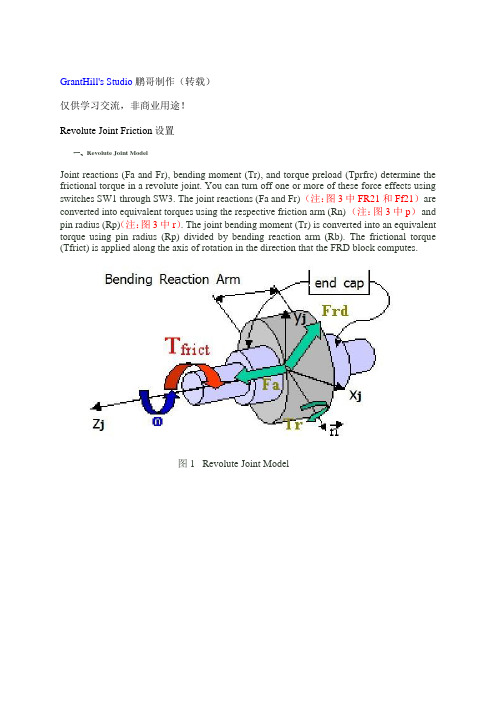
GrantHill's Studio鹏哥制作(转载)仅供学习交流,非商业用途!Revolute Joint Friction设置一、Revolute Joint ModelJoint reactions (Fa and Fr), bending moment (Tr), and torque preload (Tprfrc) determine the frictional torque in a revolute joint. You can turn off one or more of these force effects using switches SW1 through SW3. The joint reactions (Fa and Fr) (注:图3中FR21和Ff21)are converted into equivalent torques using the respective friction arm (Rn) (注:图3中p)and pin radius (Rp)(注:图3中r). The joint bending moment (Tr) is converted into an equivalent torque using pin radius (Rp) divided by bending reaction arm (Rb). The frictional torque (Tfrict) is applied along the axis of rotation in the direction that the FRD block computes.图1 Revolute Joint Model图2 Block Diagram of Revolute Joint上述是帮助文件中关于转动副中摩擦的描述。
这是一个较为复杂的模型,限于水平,这里将不对bending reaction 进行讨论。
adams运动副的高级创建
adams运动副的高级创建1.adams移动副的高级编辑过程1.1创建Adams移动副在Adams中选连接,连接类型选运动副中平面副,选择第一个物体和第二个物体,选择平面运动副作用点和平面副的移动方向,可以右键输入移动方向向量的终点坐标,移动方向向量的初始点坐标为平面运动副作用点,即可创建Adams移动副1.2给移动副增加简单数学驱动及初始条件在Adams中选择模型树下的待编辑驱动的移动副右击选择修改,选择施加驱动,其中的约束和参考点及约束名称不能修改,需要增加一个移动量表达式或选择自由,选择自由则表示需要移动副是从动件,其移动规律需要根据其它驱动来求解。
即此时的移动副只是直接限制物体运动方向,并没有直接限制物体运动大小。
移动副的驱动只能是关于时间的函数选择位置则表示对移动副对应2物体的相对位置进行主动约束,其速度和加速度根据位移求导可以得出,则其瞬时初始加速度和瞬时初始速度均无法施加,表示已经完成了移动副的所有运动约束。
此时的模型的移动副驱动要记入驱动总数量中来判断物体是否具有正常运动还是出现运动干涉或运动不确定。
例如给移动副施加x=5time^2+10*time的驱动,物体将作加速度为10,初速度10,初始位移0的匀加速直线运动。
选择速度则表示对移动副对应2物体相对速度进行主动约束,同时还要输入初始位移,其加速度和位移可以间接求出,至此完成了移动副的所有运动约束。
此时的模型的移动副驱动要记入驱动总数量中来判断物体是否具有正常运动还是出现运动干涉或运动不确定。
例如给移动副施加v=10*time+10,x0=0的驱动,物体将作加速度为10,初速度10,初始位移0的匀加速直线运动。
选择加速度则表示对移动副对应2物体相对速度进行主动约束,同时还要输入初始位移,和初始速度,其速度和位移可以间接求出,至此完成了移动副的所有运动约束。
此时的模型的移动副驱动要记入驱动总数量中来判断物体是否具有正常运动还是出现运动干涉或运动不确定。
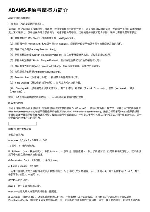
ADAMS接触与摩擦力简介
4.3.2.2接触与摩擦力1. 摩擦力(考虑是否画示意图)。
运动副一般只限制两个构件的部分自由度,在没有限制自由度的方向上,两个构件可以相对运动,在能够产生相对运动的自由度上定义摩擦力,使系统在做动力学仿真时,考虑摩擦力的存在,这样使得仿真更加符合实际,摩擦力需要设置如下参数:(1)静摩擦系数(Mu Static)和动摩擦系数(Mu Dynamic)。
(2)摩擦圆半径(Friction Arm) 和轴颈半径(Pin Radius )。
摩擦圆半径等于轴颈半径与当量摩擦系数的乘积。
(3)弯曲作用力臂(Bending Reaction Arm)。
(4)静摩擦移动速度(Stiction Transition Velocity),指在出于静摩擦状态时,运动副的最大位移。
(5)摩擦力矩预载荷(Stiction Torque Preload)。
例如由过盈装配而产生的装配压力等。
(6)引起摩擦力的因素(Input Forces to Friction)。
可以选择预载荷、方作用力或弯矩。
(7)禁用摩擦力的情况(Friction Inactive During)。
(8)Reaction Arm(反作用力力臂)。
指扭转力矩除对应的力臂。
(9)Initial Overlap(移动副的初始位移)。
指弯曲力矩对应的力臂。
(10)Overlap Will(移动副的位移变化情况)。
有三个选项,即常数(Remain Constant),增加(Increace)、减少(Decerase)。
其中,1-7为转动副摩擦的参数选项,1、4-10为移动副摩擦的参数选项。
2. 设置接触力当两个构件的表面发生接触时,就会在接触的位置参数接触力(Concact),接触力有两种计算方法,即基于回归的接触算法(Restitution-basecontact)和基于碰撞函数的接触算法(IMPACT-Function-based contact)。
接触力采用采用impact函数提供的非线性等效弹簧阻尼模型作为计算模型。
ADAMS接触与摩擦力简介
ADAMS接触与摩擦⼒简介4.3.2.2接触与摩擦⼒1. 摩擦⼒(考虑是否画⽰意图)。
运动副⼀般只限制两个构件的部分⾃由度,在没有限制⾃由度的⽅向上,两个构件可以相对运动,在能够产⽣相对运动的⾃由度上定义摩擦⼒,使系统在做动⼒学仿真时,考虑摩擦⼒的存在,这样使得仿真更加符合实际,摩擦⼒需要设置如下参数:(1)静摩擦系数(Mu Static)和动摩擦系数(Mu Dynamic)。
(2)摩擦圆半径(Friction Arm) 和轴颈半径(Pin Radius )。
摩擦圆半径等于轴颈半径与当量摩擦系数的乘积。
(3)弯曲作⽤⼒臂(Bending Reaction Arm)。
(4)静摩擦移动速度(Stiction Transition Velocity),指在出于静摩擦状态时,运动副的最⼤位移。
(5)摩擦⼒矩预载荷(Stiction Torque Preload)。
例如由过盈装配⽽产⽣的装配压⼒等。
(6)引起摩擦⼒的因素(Input Forces to Friction)。
可以选择预载荷、⽅作⽤⼒或弯矩。
(7)禁⽤摩擦⼒的情况(Friction Inactive During)。
(8)Reaction Arm(反作⽤⼒⼒臂)。
指扭转⼒矩除对应的⼒臂。
(9)Initial Overlap(移动副的初始位移)。
指弯曲⼒矩对应的⼒臂。
(10)Overlap Will(移动副的位移变化情况)。
有三个选项,即常数(Remain Constant),增加(Increace)、减少(Decerase)。
其中,1-7为转动副摩擦的参数选项,1、4-10为移动副摩擦的参数选项。
2. 设置接触⼒当两个构件的表⾯发⽣接触时,就会在接触的位置参数接触⼒(Concact),接触⼒有两种计算⽅法,即基于回归的接触算法(Restitution-basecontact)和基于碰撞函数的接触算法(IMPACT-Function-based contact)。
adams动力学仿真原理

adams动力学仿真原理一、引言动力学仿真是一种模拟真实物体运动及其相互作用的方法。
在工程领域,动力学仿真被广泛应用于设计、分析、优化以及预测产品或系统的性能。
Adams动力学仿真软件是一款功能强大的工程仿真软件,能够模拟具有复杂运动学和动力学特性的多体系统。
本文将介绍Adams动力学仿真的原理和应用。
二、运动方程和受力分析Adams基于牛顿力学和欧拉法则,通过求解运动方程来描述仿真对象的运动。
运动方程可以通过对系统中所有物体的质量、惯性矩阵以及施加在物体上的外力进行受力分析得到。
Adams提供了丰富的数学建模工具,能够精确地描述物体的几何特性、物理特性以及约束关系。
三、约束建模约束是Adams仿真中的重要概念,用于描述系统中物体之间的约束关系。
Adams支持多种约束类型,包括关节约束、接触约束、力学约束等。
通过合理地定义约束条件,可以准确地模拟物体间的接触、连接和约束。
在进行仿真前,需要根据系统的需求设置适当的约束条件,以确保仿真结果的准确性和可靠性。
四、力学属性在Adams中,物体的力学属性包括质量、惯性、刚度、阻尼等。
通过设置这些属性,可以模拟物体运动时受到的惯性力、重力、弹力、摩擦力等作用。
适当地设置力学属性,能够更加真实地模拟物体的运动行为,并实现精确的仿真分析。
五、控制器建模为了模拟真实系统中的控制装置,Adams提供了控制器建模工具。
控制器可以对系统中的物体施加不同的力或者施加控制策略来实现特定的运动目标。
通过设置适当的控制器参数和策略,可以对系统进行精确的控制和仿真分析。
六、仿真结果分析Adams提供了丰富的仿真结果分析工具,能够对仿真结果进行可视化、数据分析和优化。
通过这些工具,用户可以直观地观察仿真结果,分析系统的运动特性、力学响应以及能耗情况。
此外,Adams还支持与其他工程软件的数据交换,方便用户将仿真结果与实际工程设计相结合。
七、应用案例Adams在许多领域都得到了广泛的应用,例如汽车工业、航空航天、机械设计等。
ADAMS受力分析
ADAMS受力分析受力分析是指通过ADAMS(Automatic Dynamic Analysis of Mechanical Systems,机械系统自动动态分析)软件对机械系统进行受力分析的过程。
通过ADAMS的模型建立和动力学仿真功能,可以全面了解机械系统在运动过程中受到的各种力的大小、方向及其对机械系统的影响。
本文将介绍ADAMS受力分析的基本原理和操作步骤。
1. ADAMS受力分析的原理ADAMS受力分析基于牛顿运动定律和虚功原理,通过建立机械系统的几何约束条件和运动学关系,结合质点和刚体的动力学描述,求解机械系统在运动过程中受到的力。
具体原理如下:•牛顿运动定律:根据牛顿第二定律,物体的运动状态由施加在物体上的合力决定。
通过ADAMS可以根据机械系统中各个节点上的质点或刚体的质量、惯性矩阵和加速度等参数来计算受到的合力。
•虚功原理:虚功原理是用来处理约束系统的动力学问题的一种方法。
在ADAMS中,通过对机构约束的建立和求解,可以确定机械系统中各个节点上的受力情况。
综合应用以上原理,ADAMS受力分析能够准确地计算机械系统中各个节点上的受力情况,从而为机械系统的设计、优化和故障分析提供有力的支持。
2. ADAMS受力分析的操作步骤ADAMS受力分析的操作步骤主要包括建立模型、设置约束和求解受力等。
下面将详细介绍具体的操作步骤:步骤1:建立模型在ADAMS软件中,首先需要建立机械系统的模型。
模型可以包括刚体、质点、连杆、弹簧等各种物体和装置,具体根据所分析的机械系统而定。
建立模型的方法包括两种: - 通过ADAMS自带的几何建模工具进行建模; - 导入CAD软件中绘制的模型。
对于复杂的机械系统,通常建议使用CAD软件进行建模,然后导入ADAMS进行分析。
步骤2:设置约束在模型建立完毕之后,还需要设置机械系统中的约束条件。
约束条件包括各个节点的几何约束、运动约束和力约束等。
对于几何约束,可以通过设置节点之间的距离、角度等关系来实现,以确保机械系统在运动过程中保持一定的结构稳定性。
07-第七章 ADAMS转动和摩擦
练习 7 – 倾斜的平面
4. 选择MARKER_1 (在斜面 ramp上) 的 z 轴作为旋转轴 。
提示 : 想要更容易的选择 z 轴,一个好办法是将整个视图稍稍的旋
转一下。
Select the z-axis
ADM701, Section 1, November 2010 Copyright 2010 MSC.Software Corporation
MSC.ADAMS 初级培训教程
(ADM701 教程讲解及练习)
MSC.Software 公司
2010年11月
ADM701, Section 1, November 2010 Copyright 2010 MSC.Software Corporation
Part Number: ADAM*V2005*Z*FSP*Z*SM-ADM701-NT1
ADM701, Section 1, November 2010 Copyright 2010 MSC.Software Corporation
S1-18
练习 7 – 倾斜的平面
●
要将斜面旋转 θ = 15º :
1. 在斜面的角上的标记点上点击鼠标的右键再指向 MARKER_1 然后
选择 Modify。 2. 在 Orientation 一栏内,删除 0,0,0,输入 15,0,0。
S1-21
练习 7 – 倾斜的平面
完成旋转后的模型
● 球铰 (Spherical joints)
● 摩擦力 ( Ff)
● 与两个部件之间的接触面积无关。 ● 方向与两个部件之间相对运动速度方向相反。 ● 与正压力 (N) 成正比,比例系数为摩擦系数常数 (μ)。
Ff = μN
adams中库伦摩擦定义

adams中库伦摩擦定义好的,以下是为您创作的关于“adams 中库伦摩擦定义”的科普文章:---当我们谈到“adams 中库伦摩擦定义”时,您可能会感到有些陌生和困惑,仿佛这是一个来自遥远科学星球的神秘术语。
但别担心,让我们通过一个有趣的类比来开启这扇神秘的知识之门。
想象一下,您正在和朋友进行一场拔河比赛。
绳子在双方的拉扯下,有时候会顺畅地移动,有时候却会因为双方的力量对抗而变得僵持。
这其中,阻碍绳子顺畅移动的那种相互对抗的力量,就有点像我们今天要讲的库伦摩擦。
在 Adams 这个强大的动力学仿真软件中,库伦摩擦的定义就像是为物体之间的相对运动设置了一个“阻力规则”。
简单来说,库伦摩擦认为,当两个物体有相对运动或者有相对运动的趋势时,它们之间产生的摩擦力大小有一个上限。
这个上限取决于两个关键因素:一个是接触面之间的摩擦系数,另一个是两个物体相互挤压的正压力。
就好比在拔河比赛中,绳子与手之间的摩擦力大小,一方面取决于绳子的材质(类似于摩擦系数),另一方面也取决于您手握住绳子的力量(类似于正压力)。
摩擦系数就像是物体表面的“粗糙程度标签”。
比如,冰面很光滑,摩擦系数小,所以在冰面上行走容易滑倒;而粗糙的沙地,摩擦系数大,行走起来就会感觉到明显的阻力。
正压力呢,您可以想象成是把两个物体压在一起的力量。
比如,一个很重的箱子放在地面上,正压力就大,推动它时感受到的摩擦力也就更大;而一个很轻的小盒子,正压力小,推动时就相对轻松一些。
在实际生活中,库伦摩擦的应用场景那可真是无处不在。
比如说汽车的刹车系统。
当您踩下刹车踏板时,刹车片与刹车盘之间就会产生库伦摩擦,通过这种摩擦力来让车轮减速,最终让汽车停下来。
如果没有库伦摩擦的作用,刹车可就成了大问题,汽车就会像脱缰的野马一样难以控制。
再想想我们日常用的铅笔。
当铅笔尖在纸上划过,纸面和笔尖之间的摩擦就是库伦摩擦在起作用。
这种摩擦既让笔尖能够留下痕迹,又不会因为阻力太大而让我们写字变得费力。
ADAMS中接触的定义及参数设置
ADAMS中接触的定义及参数设置在计算机科学领域,ADAMS(Advanced Dynamic Analysis of Mechanical Systems,机械系统的高级动力学分析)是一个用于电动力学、机械学等多学科系统建模和仿真的软件。
ADAMS软件的核心理论基础是多体动力学和有限元分析。
在ADAMS中,接触是一个重要的概念,用于描述物体之间的碰撞、摩擦等相互作用。
在ADAMS中,接触被定义为两个物体之间的距离小于一个指定的阈值时发生的相互作用。
接触可以包括碰撞、接触力和摩擦等不同的形式。
ADAMS提供了一系列的接触模型和参数设置,来模拟不同类型的接触行为。
接下来我将详细介绍ADAMS中接触的定义及常用的参数设置。
1.接触定义:在ADAMS中,接触可以通过定义多种形式的接触模型来实现。
常见的接触模型包括点接触、线接触和面接触。
点接触用于描述两个物体之间的点接触,线接触描述两个物体之间的线接触,而面接触则描述两个物体之间的面接触。
2.接触力模型:- Hertz模型:用于弹性材料之间的接触力计算。
- Coulomb摩擦模型:用于描述物体之间的干摩擦行为。
- Viscous模型:用于描述物体之间的粘性摩擦行为。
- Damping模型:用于描述接触过程中的阻尼行为。
3.接触参数设置:-接触刚度:描述物体之间的刚度系数,用于计算接触力大小。
-阻尼系数:描述物体之间的阻尼行为,影响接触过程中的能量耗散。
-摩擦系数:描述物体之间的干摩擦行为,用于计算摩擦力大小。
-弹性恢复系数:描述物体在碰撞或接触中的能量损失。
-接触间隙:物体之间的实际距离和碰撞检测阈值之间的差值,决定了接触的发生时机。
根据具体的仿真需求和物体属性,可以根据实际情况设置接触参数,以使得系统的仿真结果更加准确和可靠。
总结:ADAMS中接触是描述物体之间相互作用的重要概念。
通过定义不同的接触模型和参数设置,可以模拟出不同类型的接触行为,使得系统的仿真模拟结果更加真实和准确。
adams约束介绍学习资料

-Chapter 3
3.3、运动约束
• 运动约束通过对模型施加运动来实现对模型的约束 ,一旦定义好运动后,模型就会按照所定义的运动 规律进行运动,而不考虑实现这种运动需要多大的 力或力矩。ADAMS/View定义了两种类型的运动约束 :运动副运动和点运动。
碰撞限制 -- Curve-On-Curve Cams
Curve-on-curve Cams
物件的接触碰撞固定于曲线之间,因此,碰撞 点
不会离开曲线。 移除两个DOF
构成元件 两个物件 两条曲线
一般应用于凸轮对凸轮的系统
-Chapter 33:接点介绍-
修改接点
可使用 Modify Joint 对话框 修改接点的特性
-Chapter 3
11
名称
平行约束 Parallel Axes
垂直约束 Perpendicu lar
方向约束 Orientatio n
点面约束 Inplane
点线约束 Inline
图标
说明 约束构件1的连接点,只能沿着构件2连接点标 记的Z轴运动。去除2个旋转自由度
约束构件1的Z轴始终垂直于构件2的Z轴,即: 约束构件1只能绕构件2的二个轴旋转。去除1 个旋转自由度 限定两个零件的零件坐标系坐标轴同向,不能 相对旋转,去除3个旋转自由度
限定一个零件在另一个零件的某个平面上运动 ,去除1个移动自由度
限定第一个零件沿第二个零件上的某条直线运 动,去除两个移动自由度
-Chapter 3
- 1、下载文档前请自行甄别文档内容的完整性,平台不提供额外的编辑、内容补充、找答案等附加服务。
- 2、"仅部分预览"的文档,不可在线预览部分如存在完整性等问题,可反馈申请退款(可完整预览的文档不适用该条件!)。
- 3、如文档侵犯您的权益,请联系客服反馈,我们会尽快为您处理(人工客服工作时间:9:00-18:30)。
JointsIdealized JointsAbout Idealized JointsIdealized joints connect two parts. The parts can be rigid bodies, Flexible bodies, or Point mass es. You can place idealized joints anywhere in your model.Note:The joints you can attach to flexible bodies depend on the version of Adams/Solver you are using (C++ or FORTRAN). In addition, Adams/Solver (C++) does not support pointmasses.For a summary of which joints and forces are supported on flexible bodies, see Table ofSupported Forces and Joints in the Adams/Flex online help. Also refer to the Adams/Flexonline help for more information on attaching joints and forces to flexible bodies. Adams/View supports two types of idealized joints: simple and complex. Simple joints directly connect bodies and include the following:•Revolute Joints. See Revolute Joint Tool.•Translational Joints. See Translational Joint Tool.•Cylindrical Joints. See Cylindrical Joint Tool.•Spherical Joints. See Spherical Joint Tool.•Planar Joints. See Planar Joint Tool.•Constant-Velocity Joints. See Constant-Velocity Joint Tool.•Screw Joints. See Screw Joint Tool.•Fixed Joints. See Fixed Joint Tool.•Hooke/Universal Joint. See Hooke/Universal Joint Tool.Complex joints indirectly connect parts by coupling simple joints. They include:•Gears. See Gear Joint Tool.•Couplers. See Coupler Joint Tool.You access the joints through the Joint Palette and Joint and Motion Tool Stacks.Creating Idealized JointsThe following procedure explains how to create a simple idealized joint. You can select to attach the joint to parts or spline curves. If you select to attach the joint to a curve, Adams/View creates a curve marker,Adams/View2Jointsand the joint follows the line of the curve. Learn more about curve markers with Marker Modify dialogbox help. Attaching the joint to a spline curve is only available with Adams/Solver (C++). L earn aboutswitching solvers with Solver Settings - Executable dialog box help.Note that this procedure only sets the location and orientation of the joint. If you want to set the frictionof a joint, change the pitch of a screw joint, or set initial conditions for joints, modify the joint.To create a simple idealized joint:1.From the Joint palette or tool stack, select the joint tool representing the idealized joint that youwant to create.2.In the settings container, specify how you want to define the bodies the joint connects. You canselect:• 1 Location (Bodies Implicit)• 2 Bodies - 1 Location• 2 Bodies - 2 LocationsFor more on the effects of these options, see the help for the joint tool you are creating andConnecting Constraints to Parts.3.In the settings container, specify how you want the joint oriented. You can select:•Normal to Grid - Lets you orient the joint along the current Working grid, if it is displayed, or normal to the screen.•Pick Geometry Feature - Lets you orient the joint along a direction vector on a feature in your model, such as the face of a part.4.If you selected to explicitly define the bodies by selecting 2 Bodies - 1 Location or 2 Bodies - 2Locations in Step 2, in the settings container, set First Body and Second Body to how you wantto attach the joint: on the bodies of parts, between a part and a spline curve, or between two splinecurves.ing the left mouse button, select the first part or a spline curve (splines and data element curvesare all considered curves). If you selected to explicitly select the parts to be connected, select thesecond part or another curve using the left mouse button.6.Place the cursor where you want the joint to be located (for a curve this is referred to as its curvepoint), and click the left mouse button. If you selected to specify its location on each part or curve,place the cursor on the second location, and click the left mouse button.7.If you selected to orient the joint along a direction vector on a feature, move the cursor around inyour model to display an arrow representing the direction along a feature where you want the jointoriented. When the direction vector represents the correct orientation, click the left mouse button.Modifying Basic Properties of Idealized JointsYou can change several basic properties about an Idealized joints. These include:•Parts that the joint connects. You can also switch which part moves relative to another part.3Joints •What type of joint it is. For example, you can change a revolute joint to a translational joint. Thefollowing are exceptions to changing a joint's type:•You can only change a simple idealized joint to another type of simple idealized joint or to a joint primitive.•You cannot change a joint's type if motion is applied to the joint. In addition, if a joint has friction and you change the joint type, Adams/View displays an error.•Whether or not forces that are applied to the parts connected by the joint appear graphically on the screen during an animation. Learn about Setting Up Force Graphics.•For a screw joint, you can also set the pitch of the threads of the screw (translational displacement for every full rotational cycle). Learn about screw joints.To change basic properties for a joint:1.Display the Modify Joint dialog box as explained in Accessing Modify Dialog Boxes.2.If desired, in the First Body and Second Body text boxes, change the parts that the joint connects.The part that you enter as the first body moves relative to the part you enter as the second body.3.Set Type to the type of joint to which you want to change the current joint.4.Select whether you want to display force graphics for one of the parts that the joint connects.5.For a screw joint, enter its pitch value (translational displacement for every full rotational cycle).6.Select OK.About Initial Conditions for JointsYou can specify initial conditions for revolute, translational, and cylindrical joints. Adams/View uses the initial conditions during an Initial conditions simulation, which it runs before it runs a simulation of your model.You can specify the following initial conditions for revolute, translational, and cylindrical joints:•Translational or rotational displacements that define the translation of the location of the joint on the first part (I marker) with respect to its location on the second part (J marker) in units oflength. You can set translational displacement on a translational and cylindrical joint and you can set rotational displacements on a revolute and cylindrical joint.Adams/View measures the translational displacement at the origin of the I marker along thecommon z-axis of the I and J markers and with respect to the J marker. It measures the rotational displacement of the x-axis of the I marker about the common z-axis of the I and J markers with respect to the x-axis of the J marker.•Translational or rotational velocity that define the velocity of the location of the joint on the first part (I marker) with respect to its location on the second part (J marker) in units of length per unit of time.Adams/View Joints 4Adams/View measures the translational velocity of the I marker along the common z-axis of I and J and with respect to the J marker. It measures the rotational velocity of the x-axis of the I marker about the common z-axis of the I and J markers with respect to the x-axis of the J marker.If you specify initial conditions, Adams/View uses them as the initial velocity of the joint during an assemble model operation regardless of any other forces acting on the joint. You can also leave some or all of the initial conditions unset. Leaving an initial condition unset lets Adams/View calculate the conditions of the part during an assemble model operation depending on the other forces acting on the joint. Note that it is not the same as setting an initial condition to zero. Setting an initial condition to zero means that the joint will not be moving in the specified direction or will not be displaced when the model is assembled, regardless of any forces acting on it.If you impose initial conditions on the joint that are inconsistent with those on a part that the joint connects, the initial conditions on the joint have precedence over those on the part. If, however, you impose initial conditions on the joint that are inconsistent with imparted motions on the joint, the initial conditions as specified by the motion generator take precedence over those on the joint.Setting Initial ConditionsTo modify initial conditions:1.Display the Modify Joint dialog box as explained in Accessing Modify Dialog Boxes .2.Select Initial Conditions .The Joint Initial Conditions dialog box appears. Some options in the Joint Initial Conditions dialog box are not available (ghosted) depending on the type of joint for which you are setting initial conditions.3.Set the translational or rotational displacement or velocity, and then select OK .Imposing Point Motion on a JointYou can impose a motion on any of the axes (DOF) of the idealized joint that are free to move. For example, for a translational joint , you can apply translational motion along the z-axis. Learn more About Point Motion .Note:If the initial rotational displacement of a revolute or cylindrical joint varies by anywherefrom 5 to 60 degrees from the actual location of the joint, Adams/Solver issues a warningmessage and continues execution. If the variation is greater than 60 degrees, Adams/Viewissues an error message and stops execution.Note:For translational, revolute , and cylindrical joints, you might find it easier to use the jointmotion tools to impose motion. Learn about Creating Point Motions Using the Motion Tools .5JointsTo impose motion on a joint:1.Display the Modify Joint dialog box as explained in Accessing Modify Dialog Boxes.2.Select Impose Motion.The Impose Motion(s) dialog box appears. Some options in the Impose Motion dialog box are not available (ghosted) depending on the type of joint on which you are imposing motion.3.Enter a name for the motion. Adams/View assigns a default name to the motion.4.Enter the values for the motion as explained in Options for Point Motion Dialog Box, and thenselect OK.Adding Friction to Idealized JointsYou can model both static (Coulomb) and dynamic (viscous) friction in revolute, translational, cylindrical, hooke/universal, and spherical joints.Note:Using Adams/Solver (C++), you can apply joint friction to joints if they are attached to flexible bodies; using Adams/Solver (FORTRAN), you cannot. In addition, Adams/Solver(C++) does not support point masses.For a summary of which joints and forces are supported on flexible bodies, see Table ofSupported Forces and Joints in the Adams/Flex online help. Also refer to the Adams/Flexonline help for more information on attaching joints and forces to flexible bodies.To add friction to a joint:1.Display the Modify Joint dialog box as explained in Accessing Modify Dialog Boxes.2.Select the Friction tool .The Create/Modify Friction dialog box appears. The options in the dialog box change depending on the type of joint for which you are adding friction.3.Enter the values in the dialog box for the type of joint as explained below, and then select OK.•Cylindrical Joint Options•Revolute Joint Options•Spherical Joint Options•Translational Joint Options•Universal/Hooke Joint OptionsAdams/View6JointsFriction Regime Determination (FRD)Three friction regimes are allowed in Adams/View:diagram of the friction regimes available in Adams/Solver.7JointsConventions in Friction Block DiagramsThe following tables identify conventions used in the block diagrams:•Legend for Block Diagrams identifies symbols in the diagrams.•Relationship Between the Inputs Option and Switches Used in the Block Diagrams describes the relationship between the Input Forces to Friction option in the Create/Modify Friction dialog box and the switches used in the block diagrams.Legend for Block DiagramsRelationship Between the Inputs Option and Switches Used in the Block DiagramsCylindrical Joint frictionJoint reaction (F) and reaction torque (Tm) combined with force preload (Fprfrc) and torque preload (Tprfrc) yield the frictional force and torque in a cylindrical joint. As the block diagram indicates, you can turn off one or more of these force effects using switches SW1 through SW3. The frictional force inSymbol:Description: Scalar quantityVector quantitySumming junction:c=a+bMultiplication junction:c=axbMAGMagnitude of a vector quantity ABSAbsolute value of a scalar quantity FRD Friction regime determinationSwitch:Inputs are: Symbol: Acceptable values:SW1Preload Fprfrc or Tprfc On or offSW2Reaction force f or F On or off SW3Bending moment Tr On or off SW4 Torsional moment Tn On or off All or None sets all applicable switches On or off, respectivelyAdams/View8Jointsa cylindrical joint acts at the mating surfaces of the joint. The FRD block determines the direction of thefrictional force. Based on the frictional coefficient direction, the surface frictional force is broken downinto an equivalent frictional torque and frictional force acting along the common axis of translation androtation.9JointsCylindrical Joint OptionsFor the option: Do the following:Mu Static Define the coefficient of static friction in the joint. The magnitude of thefrictional force is the product of Mu Static and the magnitude of the normalforce in the joint, for example:Friction Force Magnitude, F = µNwhere µ = Mu Static and N = normal forceThe static frictional force acts to oppose the net force or torque along theDegrees of freedom of the joint.The range is > 0.Mu Dynamic Define the coefficient of dynamic friction. The magnitude of the frictionalforce is the product of Mu Dynamic and the magnitude of the normal forcein the joint, for example:Friction force magnitude, F = µNwhere µ = Mu Dynamic and N = normal forceThe dynamic frictional force acts in the opposite direction of the velocityof the joint.The range is > 0.Initial Overlap Defines the initial overlap of the sliding parts in either a translational orcylindrical joint. The joint's bending moment is divided by the overlap tocompute the bending moment's contribution to frictional forces.The default is 1000.0, and the range is Initial Overlap > 0.Adams/View Joints 10Overlap To define friction in a cylindrical joint, Adams/Solver computes the overlapof the joint. As the joint slides, the overlap can increase, decrease, or remainconstant. You can set:•Increase indicates that overlap increases as the I marker translates in the positive direction along the J marker; the slider moves to be within thejoint.•Decrease indicates that the overlap decreases with positive translationof the joint; the slider moves outside of the joint.•Remain Constant indicates that the amount of overlap does not changeas the joint slides; all of the slider remains within the joint.The default is Remain Constant.Pin Radius Defines the radius of the pin for a cylindrical joint.The default is 1.0, and the range is > 0.Stiction TransitionVelocity Define the absolute velocity threshold for the transition from dynamic friction to static friction. If the absolute relative velocity of the joint markeris below the value, then static friction or stiction acts to make the joint stick.The default is 0.1 length units/unit time on the surface of contact in thejoint, and the range is > 0.Max StictionDeformation Define the maximum displacement that can occur in a joint once the frictional force in the joint enters the stiction regime. The slightdeformation allows Adams/Solver to easily impose the Coulombconditions for stiction or static friction, for example:Friction force magnitude < static * normal forceTherefore, even at zero velocity, you can apply a finite stiction force if yoursystem dynamics require it.The default is 0.01 length units, and the range is > 0.Friction Force Preload Define the joint's preload frictional force, which is usually caused bymechanical interference in the assembly of the joint.Default is 0.0, and the range is > 0.Friction Torque Preload Define the preload friction torque in the joint, which is usually caused bymechanical interference in the assembly of the joint.The default is 0.0, and the Range is > 0.For the option:Do the following: 搭接接头丠丠JointsFor the option: Do the following:Effect Define the frictional effects included in the friction model, either Stictionand Sliding, Stiction, or Sliding. Stiction is static-friction effect, whileSliding is dynamic-friction effect. Excluding stiction in simulations thatdon't require it can greatly improve simulation speed. The default isStiction and Sliding.Input Forces to Friction Define the input forces to the friction model. By default, all user-definedpreloads and joint-reaction force and moments are included. You cancustomize the friction-force model by limiting the input forces you specify.The inputs for a translational joint are:•Preload•Reaction Force•Bending MomentFriction Inactive During Specify whether or not the frictional forces are to be calculated during aStatic equilibrium or Quasi-static simulation.Revolute Joint FrictionJoint reactions (Fa and Fr), bending moment (Tr), and torque preload (Tprfrc) determine the frictional torque in a revolute joint. You can turn off one or more of these force effects using switches SW1 through SW3. The joint reactions (Fa and Fr) are converted into equivalent torques using the respective friction arm (Rn) and pin radius (Rp). The joint bending moment (Tr) is converted into an equivalent torque usingpin radius (Rp) divided by bending reaction arm (Rb). The frictional torque (Tfrict) is applied along the axis of rotation in the direction that the FRD block computes.Joints Revolute Joint OptionsFor the option: Do the following:Mu Static Define the coefficient of static friction in the joint. The magnitude of thefrictional force is the product of Mu Static and the magnitude of the normalforce in the joint, for example:Friction Force Magnitude, F = µNwhere µ = Mu Static and N = normal forceThe static frictional force acts to oppose the net force or torque along theDegrees of freedom of the joint.The range is > 0.Mu Dynamic Define the coefficient of dynamic friction. The magnitude of the frictionalforce is the product of Mu Dynamic and the magnitude of the normal forcein the joint, for example:Friction force magnitude, F = µNwhere µ = Mu Dynamic and N = normal forceThe dynamic frictional force acts in the opposite direction of the velocityof the joint.The range is > 0.Friction Arm Define the effective moment arm used to compute the axial component ofthe friction torque. The default is 1.0, and the range is > 0.Bending Reaction Arm Define the effective moment arm use to compute the contribution of thebending moment on the net friction torque in the revolute joint. The defaultis 1.0, and the range is > 0.Pin Radius Defines the radius of the pin.The default is 1.0, and the range is > 0.Stiction Transition Velocity Define the absolute velocity threshold for the transition from dynamic friction to static friction. If the absolute relative velocity of the joint marker is below the value, then static friction or stiction acts to make the joint stick. The default is 0.1 length units/unit time on the surface of contact in the joint, and the range is > 0.Max Stiction Deformation Define the maximum displacement that can occur in a joint once the frictional force in the joint enters the stiction regime. The slight deformation allows Adams/Solver to easily impose the Coulomb conditions for stiction or static friction, for example:Friction force magnitude < static * normal forceTherefore, even at zero velocity, you can apply a finite stiction force if your system dynamics require it.The default is 0.01 length units, and the range is > 0.Friction Torque Preload Define the preload friction torque in the joint, which is usually caused bymechanical interference in the assembly of the joint.The default is 0.0, and the Range is > 0.Effect Define the frictional effects included in the friction model, either Stictionand Sliding, Stiction, or Sliding. Stiction is static-friction effect, whileSliding is dynamic-friction effect. Excluding stiction in simulations thatdon't require it can greatly improve simulation speed. The default isStiction and Sliding.Input Forces to Friction Define the input forces to the friction model. By default, all user-definedpreloads and joint-reaction force and moments are included. You cancustomize the friction-force model by limiting the input forces you specify.The inputs for a translational joint are:•Preload•Reaction Force•Bending MomentFriction Inactive During Specify whether or not the frictional forces are to be calculated during aStatic equilibrium or Quasi-static simulation.For the option: Do the following:JointsSpherical Joint FrictionThe reaction force (F) and the preload frictional torque (Tprfrc) are the two forcing effects used in computing the frictional torque on a Spherical joint. The ball radius is used to compute an equivalent frictional torque. The FRD block determines the direction of the frictional torque.Spherical Joint OptionsFor the option: Do the following:Mu Static Define the coefficient of static friction in the joint. The magnitude of thefrictional force is the product of Mu Static and the magnitude of the normalforce in the joint, for example:Friction Force Magnitude, F = µNwhere µ = Mu Static and N = normal forceThe static frictional force acts to oppose the net force or torque along theDegrees of freedom of the joint.The range is > 0.Mu Dynamic Define the coefficient of dynamic friction. The magnitude of the frictionalforce is the product of Mu Dynamic and the magnitude of the normal forcein the joint, for example:Friction force magnitude, F = µNwhere µ = Mu Dynamic and N = normal forceThe dynamic frictional force acts in the opposite direction of the velocityof the joint.The range is > 0.Ball Radius Defines the radius of the ball in a spherical joint for use in friction-force andtorque calculations.The default is 1.0, and the range is > 0.Stiction Transition Velocity Define the absolute velocity threshold for the transition from dynamic friction to static friction. If the absolute relative velocity of the joint marker is below the value, then static friction or stiction acts to make the joint stick. The default is 0.1 length units/unit time on the surface of contact in the joint, and the range is > 0.JointsTranslational Joint FrictionJoint reaction force (F), bending moment (Tm), torsional moment (Tn), and force preload (Fprfrc) are used to compute the frictional force in a translational joint. You can individually turn off the force effects using switches SW1 through SW4.Max StictionDeformation Define the maximum displacement that can occur in a joint once the frictional force in the joint enters the stiction regime. The slightdeformation allows Adams/Solver to easily impose the Coulombconditions for stiction or static friction, for example:Friction force magnitude < static * normal forceTherefore, even at zero velocity, you can apply a finite stiction force if yoursystem dynamics require it.The default is 0.01 length units, and the range is > 0.Friction Torque Preload Define the preload friction torque in the joint, which is usually caused bymechanical interference in the assembly of the joint.The default is 0.0, and the Range is > 0.Effect Define the frictional effects included in the friction model, either Stictionand Sliding, Stiction, or Sliding. Stiction is static-friction effect, whileSliding is dynamic-friction effect. Excluding stiction in simulations thatdon't require it can greatly improve simulation speed. The default isStiction and Sliding.Input Forces to FrictionDefine the input forces to the friction model. By default, all user-definedpreloads and joint-reaction force and moments are included. You cancustomize the friction-force model by limiting the input forces you specify.The inputs for a translational joint are:•Preload•Reaction Force Friction Inactive During Specify whether or not the frictional forces are to be calculated during aStatic equilibrium or Quasi-static simulation .For the option:Do the following:The bending moment (Tm) is converted into an equivalent force using the Xs block. Similarly, torsional moment is converted into an equivalent joint force using the friction arm (Rn). Frictional force (Ffrict) is applied along the axis of translation in the direction that the FRD block computes.Joints Translational Joint OptionsFor the option: Do the following:Mu Static Define the coefficient of static friction in the joint. The magnitude of thefrictional force is the product of Mu Static and the magnitude of the normalforce in the joint, for example:Friction Force Magnitude, F = µNwhere µ = Mu Static and N = normal forceThe static frictional force acts to oppose the net force or torque along theDegrees of freedom of the joint.The range is > 0.Mu Dynamic Define the coefficient of dynamic friction. The magnitude of the frictionalforce is the product of Mu Dynamic and the magnitude of the normal forcein the joint, for example:Friction force magnitude, F = µNwhere µ = Mu Dynamic and N = normal forceThe dynamic frictional force acts in the opposite direction of the velocityof the joint.The range is > 0.Reaction Arm Define the effective moment arm of the joint-reaction torque about thetranslational joint's axial axis (the z-direction of the joint's J marker). Thisvalue is used to compute the contribution of the torsional moment to the netfrictional force.The default is 1.0, and the range is > 0.Initial Overlap Defines the initial overlap of the sliding parts in either a translational orcylindrical joint. The joint's bending moment is divided by the overlap tocompute the bending moment's contribution to frictional forces.The default is 1000.0, and the range is Initial Overlap > 0.Overlap To define friction in a cylindrical joint, Adams/Solver computes the overlapof the joint. As the joint slides, the overlap can increase, decrease, or remainconstant. You can set:•Increase indicates that overlap increases as the I marker translates in thepositive direction along the J marker; the slider moves to be within thejoint.•Decrease indicates that the overlap decreases with positive translationof the joint; the slider moves outside of the joint.•Remain Constant indicates that the amount of overlap does not changeas the joint slides; all of the slider remains within the joint.The default is Remain Constant.Stiction Transition Velocity Define the absolute velocity threshold for the transition from dynamic friction to static friction. If the absolute relative velocity of the joint marker is below the value, then static friction or stiction acts to make the joint stick. The default is 0.1 length units/unit time on the surface of contact in the joint, and the range is > 0.Max Stiction Deformation Define the maximum displacement that can occur in a joint once the frictional force in the joint enters the stiction regime. The slight deformation allows Adams/Solver to easily impose the Coulomb conditions for stiction or static friction, for example:Friction force magnitude < static * normal forceTherefore, even at zero velocity, you can apply a finite stiction force if your system dynamics require it.The default is 0.01 length units, and the range is > 0.Friction Force Preload Define the joint's preload frictional force, which is usually caused bymechanical interference in the assembly of the joint.Default is 0.0, and the range is > 0.Effect Define the frictional effects included in the friction model, either Stictionand Sliding, Stiction, or Sliding. Stiction is static-friction effect, whileSliding is dynamic-friction effect. Excluding stiction in simulations thatdon't require it can greatly improve simulation speed. The default isStiction and Sliding.For the option: Do the following:。