Section21LimitsandContinuity极限与连续

合集下载

第一章极限与连续

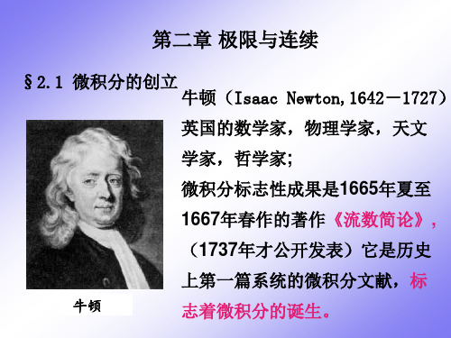
第一章极限与连续【本章导读】初等数学是用有限的方法研究常量的数学，高等数学是用极限的方法研究函数的数学.因此，极限是高等数学区别初等数学的一个标志，是初等数学向高等数学飞跃的阶梯.极限概念以及极限的思想方法将贯穿高等数学的始终.微积分学中的其他几个重要概念，如连续、导数、定积分等，都是用极限表述的，并且微积分学中的很多定理也是用极限方法推导出来的，所以准确理解极限的概念、熟练掌握极限的计算方法是学好高等数学的基础.本章将在对函数概念进行复习的基础上介绍数列与函数极限的概念、求极限的方法及函数的连续性.【学习目标】● 了解反函数、函数的单调性、奇偶性、有界性、周期性的概念；左、右极限的概念；无穷小、无穷大的概念；闭区间上连续函数的性质.● 理解函数、基本初等函数、复合函数、初等函数、分段函数的概念；函数极限的定义；无穷小的性质；函数在一点连续的概念；初等函数的连续性. ● 掌握复合函数的复合过程；极限四则运算法则.●会对无穷小进行比较；用两个重要极限求极限；判断间断点的类型；求连续函数和分段函数的极限；用极限解决经济中的问题.第一节初等函数一、函数的有关概念1．函数的定义定义1 设D 是一个数集. 如果对属于D 的每一个数x ，按照某种对应关系f ，都有确定的数值y 和它对应，那么y 就叫做定义在数集D 上的x 的函数，记为().y f x =x 叫做自变量，数集D 叫做函数的定义域，当x 取数值0x D ∈时，与0x 对应的y 的数值称为函数在点0x 处的函数值，记为0()f x ，当x 取遍D 中的一切实数值时，与它对应的函数值的集合{}=(),M y y f x x D =∈叫做函数值的值域.在函数的定义中，如对于每一个x D ∈，都有唯一确定的y 与它对应，那么这种函数称为单值函数，否则称为多值函数.如无特别说明，以后研究的函数都指单值函数.2．函数的定义域研究函数时，必须注意函数的定义域. 在实际问题中，应根据问题的实际意义来确定定义域. 对于用数学式子表示的函数，它的定义域可由函数表达式本身来确定，即要使运算有意义，一般应考虑以下几点.（1）在分式中，分母不能为零；（2）在根式中，负数不能开偶次方根；（3）在对数式中，真数不能取零和负数，底数大于零且不等于1；（4）在三角函数式中，2k k ππ+∈Z （）不能取正切，k k π∈Z （）不能取余切；（5）在反三角函数式中，要符合反三角函数的定义域；（6）如函数表达式中含有分式、根式、对数式或反三角函数式，则应取各部分定义域的交集. 例1 求下列函数的定义域.（1）214y x =- （2）lg 1x y x =-；（3）1arcsin .3x y += 解（1）要使函数有意义，必须满足24020x x ⎧-≠⎨+⎩≥，解得2x >-且2x ≠，所以函数的定义域为(2,2)(2,)-+∞U ；（2）要使函数有意义，必须满足1xx ->0，解得x >1或x <0，所以函数的定义域为(,0)(1,)-∞+∞U ；（3）要使函数有意义，必须满足111313423x x x ++-≤≤，解得-≤≤，即-≤≤，所以函数的定义域为[4,2]-.两个函数只有当它们的定义域和对应关系完全相同时，才认为这两个函数是相同的.例如，函数22sin cos y x x =+与1y =是两个相同的函数；又如，函数211x y x -=-与1y x =+是两个不同的函数.3．邻域定义 2 设0a δ∈>R ，，称开区间(,)a a δδ-+为点a 的δ邻域，记为(,)U a δ，即{}(,)(,)|U a a a x x a δδδδ=-+=-<，称a 为邻域的中心，δ为邻域的半径；将a 的δ邻域中心a 去掉后得a 的δ空心邻域，记为(,)oU a δ，即{}(,)(,)(,)|0oU a a a a a x x a δδδδ=-+=<-<U .点a 的δ邻域及点a 的δ空心邻域有时又分别简记为()U a 与().oU a4．函数的表示法常用的函数表示法有公式法（解析法）、表格法和图像法三种.有时，会遇到一个函数在自变量不同的取值范围内用不同的式子来表示.例如，函数0(),0x f x x x =-<⎪⎩≥是定义在区间(,)-∞+∞内的一个函数.在定义域的不同范围内用不同的式子来表示的函数称为分段函数.5．函数的几种特性我们已学过函数的四种特性，即奇偶性、单调性、有界性、周期性，表1-1将这四个特性做了归纳.特性定义几何特性奇偶性如函数()f x 的定义域关于原点对称，且对任意的x ，如果()f x -=()f x -，那么()f x 为奇函数；如果()f x -=()f x ，那么()f x 为偶函数奇函数的图像关于原点对称；偶函数的图像关于y 轴对称单调性对于任意的1x ，2(,)x a b ∈，且1x ＜2x ，如果1()f x ＜2()f x ，那么()f x 在(,)a b 内单调增加；如果1()f x ＞2()f x ，那么()f x 在(,)a b 内单调减少单调增函数图像沿x 轴正向上升；单调减函数图像沿x 轴正向下降有界性对于任意的(,)x a b ∈，存在M ＞0，有()f x M ≤，那么()f x 在(,)a b 内有界；如果这样的数M 不存在，那么()f x 在区间(,)a b 内无界区间(,)a b 内的有界函数的图像全部夹在直线y =M 与y =-M 之间周期性对于任意的x D ∈，存在正数l ，使()()f x l f x +=，那么()f x 为D 上的周期函数，l 叫做这个函数的周期一个以l 为周期的周期函数的图像在定义域内每隔长度为l 的区间上有相同的形状二、反函数定义3 设函数()y f x =，它的定义域是D ，值域为M ，如果对值域M 中任意一个值y ，都能由()y f x =确定D 中唯一的x 值与之对应，由此得到以y 为自变量的函数叫做()y f x =的反函数，记为1().x f y y M -=∈，在习惯上，自变量用x 表示，函数用y 表示，所以又将它改写成1()y f x -=，.x M ∈ 由定义可知，函数()y f x =的定义域和值域分别是其反函数1()y f x -=的值域和定义域．函数()y f x =和1()y f x -=互为反函数.例2 求函数32y x =-的反函数.解由32y x =-解得23y x +=，将x 与y 互换，得23x y +=，所以32y x =-（x ∈R ）的反函数是23x y +=（x ∈R ）.另外，函数()y f x =和它的反函数1()y f x -=的图像关于直线y x =对称.三、基本初等函数幂函数a y x a =∈R （）、指数函数01xy a a a =>≠（且）、对数函数log 01a y x a a =>≠（且）、三角函数和反三角函数统称为基本初等函数.现把一些常用的基本初等函数的定义域、值域、图像和特性列表，如表1-2所示.函数定义域与值域图像特性幂函数y x =(,)x ∈-∞+∞ (,)y ∈-∞+∞奇函数单调增加2y x =(,)x ∈-∞+∞[0,)y ∈+∞y =x 2偶函数在(,0)-∞内单调减少；在(0,)+∞内单调增加3y x =(,)x ∈-∞+∞ (,)y ∈-∞+∞y =x 3奇函数单调增加1y x -=(,0)(0,)x ∈-∞+∞U (,0)(0,)y ∈-∞+∞U1y x -=奇函数在(,0)-∞内单调减少；在(0,)+∞内单调减少12y x =[0,)x ∈+∞ [0,)y ∈+∞12y x =单调增加指数函数xy a=1a>（）(,)x∈-∞+∞(0,)y∈+∞y=a x（a＞1）单调增加函数定义域与值域图像特性指数函数xy a=01a<<（）(,)x∈-∞+∞(0,)y∈+∞y=a x单调减少对数函数logay x=1a>（）(0,)x∈+∞(,)y∈-∞+∞y=log a x（a＞1）单调增加logay x=01a<<（）(0,)x∈+∞(,)y∈-∞+∞y=log a x单调减少三角函数siny x=(,)x∈-∞+∞[1,1]y∈-奇函数，周期为2π，有界，在(2,2)22k kπππ-π+内单调增加，在(2,2)22k kπ3ππ+π+k∈Z（）内单调减少cosy x=(,)x∈-∞+∞[1,1]y∈-偶函数，周期为2π，有界，在(2,2)k kππ+π内单调减少，在(2,22)k kπ+ππ+πk∈Z（）内单调增加tany x=()2x k kπ≠π+∈Z(,)y∈-∞+∞奇函数，周期为π，在(,)22k kπππ-π+k∈Z（）内单调增加coty x=()x k k≠π∈Z(,)y∈-∞+∞奇函数，周期为π，在(,)k kππ+πk∈Z（）内单调减少反三角函数arcsin y x =[1,1]x ∈-[,]22y ππ∈-奇函数，单调增加，有界函数定义域与值域图像特性反三角函数arccos y x =[1,1]x ∈- [0,]y ∈π单调减少，有界arctan y x =(,)x ∈-∞+∞(,)22y ππ∈-奇函数，单调增加，有界arccot y x =(,)x ∈-∞+∞(0,)y ∈π单调减少，有界四、复合函数、初等函数1．复合函数定义4 设y 是u 的函数()y f u =；而u 又是x 的函数()u x ϕ=，其定义域为数集A .如果在数集A 或A 的子集上，对于x 的每一个值所对应的u 值，都能使函数()y f u =有定义，那么y 就是x 的函数. 这个函数叫做函数()y f u =与()u x ϕ=复合而成的函数，简称为x 的复合函数，记为[]()y f x ϕ=，其中u 叫做中间变量，其定义域为数集A 或A 的子集.例如，2tan y x =是由2y u =与tan u x =复合而成的函数；函数ln(1)y x =-是由ln y u =与1u x =-复合而成的函数，它们都是x 的复合函数.注意：（1）不是任何两个函数都可以复合成一个函数的.例如arcsin y u =与22u x =+就不能复合成一个函数.（2）复合函数也可以有两个以上的函数复合构成.例如2u y =，1sin u v v x==，，由这三个函数可得复合函数1sin2xy =，这里u 和v 都是中间变量.例3 指出下列各复合函数的复合过程. （1）21y x =+；（2）arcsin(ln )y x =；（3）2sin e x y =.解（1）21y x =+是由y u =与21u x =+复合而成；（2）arcsin(ln )y x =是由arcsin y u =与ln u x =复合而成；（3）2sin e x y =是由2e sin u y u v v x ===，，复合而成.2．初等函数定义5 由基本初等函数和常数经过有限次四则运算以及有限次的复合步骤所构成的，并能用一个式子表示的函数称为初等函数.例如，3322221lncos tan e sin(21)1x x y x y x y y x x -====++，，，都是初等函数.在初等函数的定义中，明确指出是用一个式子表示的函数，如果一个函数必须用几个式子表示时，它就不是初等函数.例如，2,01()1,1x x g x x x ⎧⎪=⎨+>⎪⎩≤≤就不是初等函数，而称为非初等函数.五、建立函数关系举例在解决实际问题时，通常要先建立问题中的函数关系，然后进行分析和计算. 下面举一些简单的实际问题，说明建立函数关系的过程.例4 某工厂生产人造钻石，年生产量为x kg ，其固定成本为312万元，每生产1kg 人造钻石，可变成本均匀地增加50元，试将总成本C 总（单位：元）和平均单位kg 成本C 均（单位：元/kg ）表示成产量x （单位：kg ）的函数.解由于总成本=固定成本+可变成本，平均成本=总成本/产量，所以C 总=3 120 000+50x ，C 均=312000050312000050.x x x+=+ 例5 某运输公司规定货物的吨千米运价为：在a 千米以内，每千米k 元；超过a 千米时超过部分每千米45k 元.求运价m 与里程s 之间的函数关系.解根据题意可列出函数关系如下：,04(),5ks s a m ka k s a s a <⎧⎪=⎨+->⎪⎩≤. 这里运价m 和里程s 的函数关系是用分段函数表示的，定义域为(0,)+∞.例6 将直径为d 的圆木料锯成截面为矩形的木材（见图1-1），列出矩形截面两条边长之间的函数关系.解设矩形截面的一条边长为x ，另一条边长为y ，由勾股定理得222x y d +=.解出22y d x =±-，由于y 只能取正值，所以22y d x =-，这就是矩形截面的两条边长之间的函数关系，它的定义域为(0,d ).图 1-1一般地，建立函数关系式应根据题意，先分析问题中哪些是变量，哪些是常量；在变量中，哪个是自变量，哪个是函数，并用不同的字母表示；再根据问题中给出的条件，运用数学、物理等方面的知识，确定等量关系；必要时，还须根据所给条件，确定关系式中需要确定的常数或删除式中出现的多余变量，从而得出函数关系式，并根据题意写出函数的定义域.如果变量之间的关系式在自变量的各个取值范围内各不相同，则需进行分段考察，并将结果写成分段函数.思考题1．分段函数的图像如何作？作出分段函数1,0()2,0x x x f x x +<⎧⎪=⎨⎪⎩≥的图像.2．几个函数能复合成一个函数的条件是什么？ln cos (,)2y u u x x π==∈π，，能否复合成一个函数？为什么？3. 基本初等函数的特点是什么？习题1-11．下列各题中所给的两个函数是否相同？为什么？（1）y x y ==和（2）2y x y ==和；（3）2422x y x y x-=-=+和；（4）1ln(1)2y y x ==-.2．求下列函数的定义域. （1）y（2）y =（3）2232y x x =-+；（4）1lg1xy x+=-；（5）1lg(1)y x =+；（6）y =.3．设()(0)2(3)5f x ax b f f =+=-=，，，求(1)f 和(2)f . 4．已知2(1)32()f x x x f x -=-+，求. 5．判断下列函数的奇偶性. （1）42()23f x x x =-+；（2）2()cos g x x x =；（3）1()(e e )2x x f x -=+；（4）()1x xg x a =-.6．证明函数1y x=在区间(1-,0)内单调减少.7．将下列各题中的y 表示为x 的函数. （1）21y u x =-；（2）e sin ln u y u v v x ===，，.8．指出下列函数的复合过程. （1）y = （2）21sin y x=；（3）1ln(sine)x y +=；（4）1cot 5xy =.9．火车站收取行李费的规定如下：当行李不超过50kg 时，按基本运费计算，每公斤收费0.15元；当超过50kg 时，超重部分按每公斤0.25元收费.试求运费y （元）与重量x （kg ）之间的函数关系式，并作出这个函数的图像.10．拟建一个容积为8 000立方米、深为8米的长方体水池，池底造价比池壁造价贵一倍，假定池底每平方米的造价为a元，试将总造价表示成底的一边长的函数，并确定此函数的定义域.第二节数列的极限一、数列极限的定义根据数列的概念，现在进一步考察当自变量n无限增大时，数列()nx f n=的变化趋势，先看下面两个数列：（1）11111,,,,,,248162nL L；（2）1143(1)2,,,,,,.234nnn-+-L L为清楚起见，把这两个数列的前几项在数轴上表示出来，分别如图1-2和图1-3所示.图1-2图1-3由图1-2可以看出，当n无限增大时，表示数列12n nx=的点逐渐密集在0x=的右侧，即数列nx无限接近于0；由图1-3可以看出，当n无限增大时，表示数列1(1)nnnxn-+-=的点逐渐密集在1x=的附近，即数列nx无限接近于1.归纳这两个数列的变化趋势，可知当n无限增大时，nx都分别无限接近于一个确定的常数.一般地，有如下定义.定义6如果当n无限增大时，数列{}n x无限接近于一个确定的常数a，那么a就叫做当n 趋向无穷大时数列{}n x的极限，记为limn nnx a n x a→∞=→∞→或当时，.因此，数列（1）和数列（2）的极限分别记为11(1)lim0lim12nnn nnn-→∞→∞+-==；.例7 观察下列数列的变化趋势，写出它们的极限.（1）1n x n =；（2）212n x n =-；（3）1(1)3n n n x =-；（4）3n x =-.解列表考察这四个数列的前几项，以及当n →∞时，它们的变化趋势如表1-3所示.表 1-3由表1-3中各数列的变化趋势，根据数列极限的定义可知，（1）1lim lim 0n n n x n →∞→∞==；（2）21lim lim(2)2n n n x n→∞→∞=-=；（3）1lim lim(1)03n n n n n x →∞→∞=-=；（4）lim lim(3) 3.n n n x →∞→∞=-=-注意：并不是任何数列都有极限.例如，数列2n n x =，当n 无限增大时，n x 也无限增大，不能无限接近于一个确定的常数，所以这个数列没有极限.又如，数列1(1)n n x +=-，当n 无限增大时，n x 在1与-1 两个数上来回跳动，不能无限接近于一个确定的常数，所以这个数列也没有极限.没有极限的数列，也说数列的极限不存在.二、数列极限的四则运算设有数列lim lim n n n n n n x y x a y b →∞→∞==和，且，，则（1）lim()lim lim n n n n n n n x y x y a b →∞→∞→∞±=±=±；（2）lim()lim lim n n n n n n n x y x y a b →∞→∞→∞⋅=⋅=⋅；（3）limlim0.lim n n n n n nn x x a b y y b →∞→∞→∞==≠（）这里（1）和（2）可推广到有限个数列的情形. 推论若lim C n n x k →∞∈N 存在，为常数，，则（1）lim(C )C lim n n n n x x →∞→∞⋅=⋅；（2）lim()(lim )k k n n n n x x →∞→∞=.例8 已知lim 5lim 2n n n n x y →∞→∞==，，求（1）lim(3)n n x →∞；（2）lim5nn y →∞；（3）lim(3).5nn n y x →∞-解（1）lim(3)3lim 3515n n n n x x →∞→∞==⨯=；（2）12limlim 555n n n n y y →∞→∞==；（3）23lim(3)lim(3)lim 15145555n n n n n n n y y x x →∞→∞→∞-=-=-=.例9 求下列各极限.（1）213lim(4)n n n →∞-+；（2）2231lim .1n n n n →∞-++ 解（1）221311lim(4)lim 4lim 3lim n n n n n nn n →∞→∞→∞→∞-+=-+40304=-+⨯=；（2）22222211113lim3lim lim 31lim lim 1111lim lim1n n n n n n n n n n n n n n n n →∞→∞→∞→∞→∞→∞→∞-+-+-+==+++300 3.01-+==+ 三、无穷递缩等比数列的求和公式等比数列211111,,,,,n a a q a q a q -L L ，当1q <时，称为无穷递缩等比数列.现在来求它的前n 项的和n S n →∞当时的极限.1111(1)(1)lim lim lim lim(1)(lim1lim ).1111n n n n n n n n n n n n a q a q a aS S q q q q q q →∞→∞→∞→∞→∞→∞--=∴==⋅-=-----Q ，111lim 0lim (10)11n n n n a aq q S q q→∞→∞<=∴=-=--Q 当时，，.我们把无穷递缩等比数列前n 项的和当n →∞时的极限叫做这个无穷递缩等比数列的和，并用符号S 表示，从而有公式11a S q=-. 这个公式叫做无穷递缩等比数列的求和公式.例10 求数列1111,,,,,2482n L L 各项的和.解 112q =<因为，所以它是无穷递缩等比数列，因此有121112S ==-.思考题1．“{},n n x n x A 对数列如果当无限增大时，越来越接近于常数，则称数列{}n x 以A 为极限”，这种说法正确吗？2．数列1,2,131411,,,,,,,2233n n n+L L 是否有极限？习题1-21．观察下列数列当n →∞时的变化趋势，写出极限.（1）12n x n =；（2）1(1)n n x n =-；（3）213n x n =+；（4）11n n x n -=+；（5）1110n n x =-；（6） 5.n x =-2．已知1lim 2n n x →∞=，1lim 2n n y →∞=-，求下列各极限.（1）lim(23)n n n x y →∞+；（2）lim .nnn n x y x →∞- 3．求下列各极限.（1）1lim(3)n n→∞-；（2）53lim n n n→∞+；（3）224lim 1n n n →∞-+；（4）33321lim 8n n n n →∞-+-；（5）221lim(3)n n n →∞-+；（6）51lim(3)(2)2n n n→∞--；（7）2221lim 1n n n →∞+-；（8）23lim()1n n n n →∞--+；（9）21lim 12n n n →∞-+；（10）123lim().22n n nn →∞++++-+L 4．求下列无穷递缩等比数列的和.（1）113,1,,,39L ；（2）1111,,,,248--L ；（3）231,,,,(1).x x x x --<L第三节函数的极限本节将讨论一般函数()y f x =的极限，主要研究以下两种情形.（1）当自变量x x 的绝对值无限增大，即x 趋向无穷大（记为x →∞）时，函数()f x 的极限.（2）当自变量x 任意接近于0x ，即x 趋向于定值0x （记为0x x →）时，函数()f x 的极限.一、当x →∞时，函数()f x 的极限先看下面的例子：考察当x →∞时，函数1()f x x=的变化趋势.由图1-4可以看出，当x 的绝对值无限增大时，()f x 的值无限接近于零.即当x →∞时，()0f x →.对于这种当x →∞时，函数()f x 的变化趋势，给出下面的定义.定义7 如当x 的绝对值无限增大（即x →∞）时，函数图 1-4()f x 无限接近于一个确定的常数A ，那么A 就叫做函数()f x x →∞当时的极限，记为lim ()().x f x A x f x A →∞=→∞→或当时，根据上述定义可知，当1()x f x x→∞=时，的极限是0，可记为 1lim ()lim 0.x x f x x→∞→∞== 注意：自变量x 的绝对值无限增大指的是x 既取正值而无限增大（记为x →+∞），同时也取负值而绝对值无限增大（记为x →-∞）.但有时x 的变化趋势只能或只需取这两种变化中的一种情形.下面给出当x x →+∞→-∞或时函数极限的定义.定义8 如果当x x →+∞→-∞（或）时，函数()f x 无限接近于一个确定的常数A ，那么A 就叫做函数()f x x x →+∞→-∞当（或）时的极限，记为()lim ()().x x f x A x x f x A →-∞→+∞=→+∞→-∞→或当（）时，例如，如图1-5所示，lim arctan lim arctan .22x x x x →+∞→-∞ππ==-及由于当arctan x x y x →+∞→-∞=和时，函数不是无限接近于同一个确定的常数，所以limarctan x x →∞不存在.一般地，lim ()x f x A →∞=的充分必要条件是lim ()lim ().x x f x f x A →+∞→-∞==例11 求lim e lim e x x x x -→-∞→+∞和.解如图1-6所示，可知lim e 0lim e 0.x x x x -→-∞→+∞==，y =e -xy =e x图 1-5 图 1-6例12 讨论当x →∞时，函数arccot y x =的极限.解因为lim artcot 0lim arccot x x x x →+∞→-∞==π，，虽然lim arccot x x →+∞和lim arccot x x →-∞都存在，但不相等，所以lim arccot x x →-∞不存在.二、当0x x →时，函数()f x 的极限定义9 如果当x 无限接近于定值000x x x x x →，即（可以不等于）时，函数()f x 无限接近于一个确定的常数A ，那么A 就叫做函数0()f x x x →当时的极限，记为lim ()x x f x A →= 或当0x x →时，().f x A →注意：（1）在上面的定义中，0x x →“”表示既从0x 的左侧同时也从0x 的右侧趋近于0x ；（2）定义中考虑的是当0x x →时，()f x 的变化趋势，并不考虑0()f x x 在点是否有定义. 例13 考察极限0lim C C x x →（为常数）和0lim .x x x →解设()C ()f x x x ϕ==，.0()C lim ()lim C C.x x x x x x f x f x →→→∴==Q 当时，的值恒等于，000()lim ()lim .x x x x x x x x x x x ϕϕ→→→∴==Q 当时，的值无限接近于，三、当0x x →时，()f x 的左极限与右极限前面讨论的当0x x →时函数的极限中，0x x 既从的左侧无限接近于0x （记为00x x →-或0x -），也从0x 的右侧无限接近于0x （记为00x x →+或+0x ）.下面再给出当00x x x x -+→→或时函数极限的定义：定义10 如果当0x x -→时，函数()f x 无限接近于一个确定的常数A ，那么A 就叫做函数()f x 当0x x →时的左极限，记为00lim ()(0).x x f x A f x A -→=-=或如果当0()x x f x +→时，函数无限接近于一个确定的常数A ，那么A 就叫做函数()f x 当0x x →时的右极限，记为00lim ()(0).x x f x A f x A +→=+=或一般地，0lim ()x x f x A →=的充分必要条件是0lim ()lim ().x x x x f x f x A -+→→==例14 讨论函数1,0()0,01,0x x f x x x x -<⎧⎪==⎨⎪+>⎩，当0x →时的极限. 解作出这个分段函数的图像（见图1-7），由图可知函数()f x 当0x →时的左极限为lim ()lim(1)1x x f x x --→→=-=-，右极限为00lim ()lim(1)1x x f x x ++→→=+=. 因为当0x →时，函数()f x 的左极限与右极限虽各自存在但不相等，所以极限0lim ()x f x →不存在.例15 讨论函数2111x y x x -=→-+当时的极限.解函数的定义域为(,1)(1,)-∞--+∞U ；因为1x ≠-，所以2111x y x x -==-+.作出这个函数的图像（见图1-8），由图1-8可知，2111lim lim (1)21x x x x x --→-→--=-=-+；2111lim lim (1)21x x x x x ++→-→--=-=-+；由于221111lim lim 11x x x x x x -+→-→---=++，所以211lim 21x x x →--=-+.图 1-7 图 1-8思考题1．若0lim ()x x f x →存在，则0()f x 必存在，对吗？两者之间是否有关系？2．由lim ()1x f x →+∞=，画图说明曲线()y f x =的几何特征.习题1-31．观察并写出下列极限.（1）21lim x x→∞；（2）lim 2x x →-∞；（3）lim 10x x →-∞；（4）1lim ()2x x →+∞；（5）1lim ()10xx →+∞；（6）1lim (2).x x →∞+2．观察并写出下列极限.（1）0limtan x x →；（2）2limsin x x π→；（3）1limln x x →；（4）0lim 2x x →；（5）239lim3x x x →--+；（6）22lim(2)x x →-；（7）4lim tan x x π→；（8）23lim(68).x x x →-+3．设21,0()1,0x x f x x x ⎧-⎪=⎨+⎪⎩≤＞，画出图像，并求当0()x f x →时的左右极限，从而说明在0()x f x →时，的极限是否存在.4．设1,0()2,0xx x f x x +⎧⎪=⎨⎪⎩＜≥，求当0()x f x →时的左右极限，并指出当0x →时极限是否存在.5．求()0x f x x x=→当时的左右极限，并指出当0x →时极限是否存在.6．讨论函数2,0()2,013,1x x f x x x x ⎧⎪=⎨⎪-+⎩＜≤＜≥，当01x x →→和时是否有极限？ 7．证明函数21,1()1,11,1x x f x x x ⎧+⎪==⎨⎪-⎩＜＞，当1x →时极限不存在. 第四节极限的运算与数列极限相仿，比较复杂的函数极限也需要用到极限的运算法则来进行计算.下面给出函数极限的四则运算法则（证明从略）.设0lim ()lim ()x x x x f x A g x B →→==，，则（1）[]00lim ()()lim ()lim ()x x x x x x f x g x f x g x A B →→→±=±=±；（2）[]0lim ()()lim ()lim ().x x x x x x f x g x f x g x A B →→→⋅=⋅=⋅特别地，有0limC ()C lim ()C x x x x f x f x A →→=⋅=（C 为常数）；[]00lim ()lim ()nnn x x x x f x f x A →→⎡⎤==⎢⎥⎣⎦（n 是正整数）.（3）000lim ()()lim()lim ()x x x x x x f x f x A g x g x B→→→==（0B ≠）. 上述极限运算法则对于00x x -+，，x x x →∞→+∞→-∞，，的情形也是成立的，而且法则（1）和法则（2）可以推广到有限个具有极限的函数的情形. 例16 求22lim(326)x x x →-+.解 2222222lim(326)3[lim ]2lim lim63222614x x x x x x x x →→→→-+=-+=⨯-⨯+=.例17 求22125lim7x x x x →-++.解当1x →时，分母的极限不为0，因此应用法则（3），得22211112221111lim(25)lim lim2lim5251251lim 7lim(7)lim lim7172x x x x x x x x x x x x x x x x x →→→→→→→→-+-+-+-+====++++. 例18 求233lim9x x x →--.解当3x →时，分母极限为0，不能应用法则（3），在分式中约去极限为零的公因子3x -，所以323333lim1311lim lim 93lim lim36x x x x x x x x x →→→→→-===-++.例19 求211lim (1)(2).x x x →∞⎡⎤+-⎢⎥⎣⎦解 221111lim (1)(2)lim(1)lim(2)x x x x x x x →∞→∞→∞⎡⎤+-=+⋅-⎢⎥⎣⎦211lim1lim lim2lim x x x x x x →∞→∞→∞→∞⎡⎤⎡⎤=+⋅-⎢⎥⎢⎥⎣⎦⎣⎦(10)(20) 2.=+-=例20 求3232342lim 753x x x x x →∞-++-.解先用3x 同除分子及分母，然后取极限，得3233323342423lim3lim lim 342lim lim 53537537lim7lim lim x x x x x x x x x x x x x x x x x xx x →∞→∞→∞→∞→∞→∞→∞→∞-+-+-+==+-+-+-340203750307-⨯+⨯==+⨯-⨯. 例21 求232321lim .25x x x x x →∞---+解先用3x 同除分子及分母，然后取极限，得2232332333211113lim 2lim lim 3210lim lim 0.15112522lim2lim 5lim x x x x x x x x x x x x x x x x x x x xx x →∞→∞→∞→∞→∞→∞→∞→∞------====-+-+-+ 例22 求2123(1)lim.n n n →∞++++-L 解因为123(1)(1)2nn n ++++-=-L ，所以22(1)123(1)111112lim lim lim lim(1).222n n n n nn n n n n n n →∞→∞→∞→∞-++++--===-=L 例23 求21lim .41n n n →∞-+解 22222222211111lim (lim )212122222lim lim lim lim 1121412111(lim )222n n n n n n n n n n n n n n n n n n n nn →∞→∞→∞→∞→∞→∞→∞-----====+++++00.1== 思考题1．22lim(3)lim 3lim 0x x x x x x x →∞→∞→∞-=-=∞-∞=，计算是否正确？2．为什么说22222lim 4lim2lim(2)0x x x x x x x →→→===∞--是错误的？习题1-41．求下列各极限.（1）21lim(45)x x x →-+；（2）22lim (352)x x x →--+；（3）22lim 1x x x →+-；（4）2x ；（5）222lim 1x x x →---；（6）02lim(1)3x x →--；（7）22125lim 1x x x x →-+++；（8）22121lim.1x x x x →-+- 2．求下列各极限.（1）221lim 21x x x x →∞---；（2）442321lim 25x x x x x →∞++++；（3）242lim 31x x xx x →∞+-+；（4）324223lim .325x x x xx x →∞+-+- 3．求下列各极限.（1）224lim 2x x x →--+；（2）2565lim5x x x x →-+-；（3）22468lim54x x x x x →-+-+；（4）23121lim x x x x x→-+-；（5）322042lim 32x x x xx x →-++；（6）330()lim h x h x h→+-；（7）2316lim().39x x x →--- 4．求下列各极限.（1）232248lim 21x x x x x →∞-++-；（2）3381lim 651x x x x →∞--+；（3）152lim 51x x x +→+∞++；（4）111lim(1)242n n →∞++++L ；（5）(1)lim.(2)(3)n n n n n →∞+++ 第五节无穷小与无穷大研究函数的变化趋势时，经常遇到两种情形：一是函数的绝对值“无限变小”；二是函数的绝对值“无限变大”.下面分别介绍这两种情形.一、无穷小1．无穷小的定义定义11 如果当0()x x x f x →→∞（或）时，函数的极限为零，那么函数()f x 叫做当0x x → x →∞（或）时的无穷小量，简称无穷小. 例如，因为1lim(1)0x x →-=，所以函数11.x x -→是当时的无穷小又如，因为1lim0x x→∞=，所以函数1x是当x →∞时的无穷小. 注意：（1）说一个函数()f x 是无穷小，必须指明自变量x 的变化趋势，如函数1x -是当1x →时的无穷小，而当x 趋向其他数值时，1x -就不是无穷小.（2）不要把一个绝对值很小的常数（如1000001000000.000010.00001-或）说成是无穷小.（3）常数中只有“0”可以看成是无穷小，因为0()lim 00.x x x →∞→=2．无穷小的性质无穷小运算时除了可以应用极限运算法则外，还可以应用以下一些性质进行运算. 性质1 有限个无穷小的代数和是无穷小. 性质2 有界函数与无穷小的乘积是无穷小. 性质3 有限个无穷小的乘积是无穷小. 以上各性质证明从略.例24 求01lim sin .x x x→解因为0lim 0x x →=，所以0x x →是当的无穷小.而11sin 1sin x x≤，所以是有界函数. 由无穷小的性质2，可知1lim sin0.x x x→= 3．函数极限与无穷小的关系下面的定理将说明函数、函数的极限与无穷小三者之间的重要关系.定理 1 在自变量的同一变化过程0lim ()x x x f x A →→∞=（或）中，的充分必要条件是：()f x A α=+，其中A 为常数，α为无穷小（证明从略）.这里“lim ”符号下面下标为0x x x →→∞或，表示所述结果对两者都适用，以后不再说明.二、无穷大1．无穷大的定义定义 12 如果当0()x x x f x →→∞（或）时，函数的绝对值无限增大，那么函数()f x 叫做当0x x x →→∞（或）时的无穷大量，简称无穷大. 如果函数0()f x x x x →→∞当（或）时为无穷大，那么它的极限是不存在的.但为了描述函数的这种变化趋势，也说“函数的极限是无穷大”，并记为()lim ().x x x f x →∞→=∞如果在无穷大的定义中，对于0x 左右近旁的x （或对于绝对值相当大的x ），对应的函数值都是正的或都是负的，就分别记为()lim ()x x x f x →∞→=+∞，0()lim ().x x x f x →∞→=-∞例如，lim e x x →+∞=+∞，0lim ln .x x →+=-∞注意：（1）说一个函数()f x 是无穷大，必须指明自变量的变化趋势，如函数1x是当0x →时的无穷大.（2）无穷大是变量，不要把绝对值很大的常数（1000000100000000如或1000000100000000-）说成是无穷大.2．无穷大与无穷小的关系一般地，无穷大与无穷小之间有以下倒数关系. 在自变量的同一变化过程中，如果()f x 为无穷大，则1()f x 是无穷小；反之，如果()f x 为无穷小，且1()0()f x f x ≠，则为无穷大. 下面利用无穷大与无穷小的关系来求一些函数的极限.例25 求极限14lim.1x x x →+- 解当1x →时，分母的极限为零，所以不能应用极限运算法则（3），但因为11lim04x x x →-=+，所以14lim.1x x x →+=∞-例26 求2lim(32).x x x →∞-+解因为2lim lim3x x x x →∞→∞和都不存在，所以不能应用极限的运算法则，但因为21lim32x x x →∞=-+221lim 0321x x x x→∞=-+，所以2lim(32).x x x →∞-+=∞例27 求32225lim .7x x x x →∞-++解因为分子及分母的极限都不存在，所以不能应用极限运算法则，但因为22333232337177lim lim lim 01525252x x x x x x x x x x x x x x x→∞→∞→∞+++===-+-+-+，所以 32225lim .7x x x x →∞-+=∞+归纳第四节中例21、例22及本节的例27，可得以下的一般结论，即当0000a b ≠≠，时有0,0,,a n mb n m n m⎧=⎪⎪⎨>⎪⎪∞<⎩当当当例28 求32112lim().28x x x →--++解因为23222112(24)12(2)(4)4.28(2)(24)(2)(24)24x x x x x x x x x x x x x x x -+-+---===+++-++-+-+ 1201212012lim m m m m n n n x n a x a x a x a b x b x b x b ----→∞++++=++++L L所以 3222112461lim()lim .28244442x x x x x x x →-→----===-++-+++ 例29 求11110e e lim.e exx x xx-→+--+解令111e 0e.xxt x t t -=→+→+∞=，则当时，，同时从而 1121102111e e limlim lim 1.111e exx x t t xxt t t t t t-→+→+∞→+∞----===+++三、无穷小的比较已经知道，两个无穷小的代数和及乘积仍然是无穷小. 但是两个无穷小的商却会出现不同的情况. 例如，当0x →时，x 、3x 、2x 都是无穷小，而20lim 03x x x→=， 203lim x x x →=∞， 03lim 3.x x x →=两个无穷小之比的极限的各种情况，反映了不同的无穷小趋向零的快慢程度. 当0x →时，2x 比3x 更快地趋向零，反过来23x x 比较慢地趋向零，而3x x 与趋向零的快慢相仿.下面就以两个无穷小之商的极限所出现的各种情况来说明两个无穷小之间的比较.定义 13 设αβ和都是在同一个自变量的变化过程中的无穷小，又lim βα也是在这个变化过程中的极限.（1）如果lim 0βα=，就说βα是比较高阶的无穷小.（2）如果lim βα=∞，就说βα是比较低阶的无穷小.（3）如果lim C C βα=（为不等于零的常数），就说βα与是同阶无穷小.（4）如果lim 1βα=，就说βα与是等价无穷小，记为.αβ～显然，等价无穷小是同阶无穷小的特例，即C 1=的情形. 以上定义对于数列的极限也同样适用. 根据以上定义，可知当0x →时，23x x 是比较高阶的无穷小，23x x 是比较低阶的无穷小，3x 是与x 同阶无穷小.例30 比较当0x →时，无穷小2111x x x---与阶数的高低. 解因为22220000111(1)(1)11limlim lim lim 1(1)(1)1x x x x xx x x x x x x x x x →→→→---+--====---，所以211~1x x x---，即当0x →时，2111x x x---与是等价无穷小. 思考题1．指出函数()f x 是无穷小或无穷大的变化过程. 2．为什么说10lime xx →=+∞是错误的，请予以验证.习题1-51．以下各数列中，哪些是无穷小？哪些是无穷大？（1）1111,,,,,3521n -L L ；（2）1111,,,,,3721n -L L ；（3）1,3,5,,12,n ----L L ；（4）1111,,,,(1),2482n n ---L L ；（5）1111,,,,,122334(1)n n ⨯⨯⨯+L L ；（6）21,4,9,,,.n L L 2．下列函数在自变量怎样变化时是无穷小？无穷大？（1）31y x =；（2）13cot 4ln .1y y x y x x ===+；（）；（） 3．求下列各极限.（1）0lim(sin )x x x →+；（2）0lim3sin x x →；（3）1lim(1)cos x x x →-；（4）2sin lim x xx→∞；（5）1lim 1x xx →-；（6）32222lim.(2)x x x x →+-4．当211x x x→∞时，和相比，哪一个是较高阶的无穷小？5．求下列各极限.（1）23lim 21x x x x →∞-+；（2）32428lim 31x x x x →∞-++；（3）3321lim 52x x x x x →∞++--；（4）2lim()cos()22x x x π→ππ--；（5）201lim sin x x x→.6．证明：当23693x x x x →-+++时，是比较高阶的无穷小. 7．当1x →时，无穷小211(1)2x x --和是否同阶？是否等价？第六节两个重要极限一、极限0sin lim1x xx→= 我们先列表考察当0x →时，函数sin xx的变化趋势，如表1-4所示. 表 1-4由表1-4可见，当sin 01xx x→→时，.可以证明，000sin sin sin limlim 1lim 1.x x x x x xx x x →+→-→===，所以例31 求0sin 2lim.x xx → 解 000sin 2sin 2sin 2lim lim(2)2lim 22x x x x x xx x x→→→=⋅=.设200t x x t =→→，则当时，.所以00sin 2sin lim 2lim 21 2.x t x t x t→→==⨯= 例32 求0tan lim.x xx → 解 0000tan sin 1sin 1limlim()lim lim 1.cos cos x x x x x x x x x x x x→→→→=⋅=⋅= 例33 求201cos lim.x xx →- 解 22220002sin sin1cos 1122lim lim lim .222x x x x x x x x x →→→⎡⎤⎢⎥-===⎢⎥⎢⎥⎣⎦例34 求2cos lim .2αααπ→π- 解因为cos sin()2ααπ=-，所以22sin()cos 2lim lim .22ααααααππ→→π-=ππ-- 设0.22t t ααππ=-→→，则当时，所以02cos sin lim lim 1.2t t t αααπ→→==π- 在例31、例34中使用了代换，其实在运算熟练后不必都要经过变量代换化成第一个重要极限形式.二、极限1lim(1)e x x x→∞+= 先列表考察当x x →+∞→-∞及时，函数1(1)x x+的变化趋势，分别如表1-5和表1-6所示.表 1-5表 1-6从表1-5和表1-6可以看出，当x x →+∞→-∞或时，函数1(1)x x+的对应值无限地趋近于一个确定的数2.71828.L可以证明，当x x →+∞→-∞及时，函数1(1)x x+的极限都存在而且相等，我们用e 表示这个极限值，即1lim(1) e.x x x→∞+= （1.1）这个数e 是个无理数，它的值是：e 2.718281828459045.=L在式（1.1）中，设10z x z x=→∞→，则当时，，于是式（1.1）又可以写成1lim(1) e.zz z →+= （1.2）式（1.1）和式（1.2）可以看成一个重要极限的两种不同形式.例35 2lim(1)x x x→∞+.解先将21x+写成112x +形式，从而2222222111lim(1)lim(1)lim(1)lim(1)e .222x x x x x x x x x x x x →∞→∞→∞→∞⎡⎤⎡⎤⎢⎥⎢⎥+=+=+=+=⎢⎥⎢⎥⎢⎥⎢⎥⎣⎦⎣⎦例36 求极限1lim(1).x x x→∞-解 1111lim(1)lim(1)lim (1)x x x x x x x x x --→∞→∞→∞⎡⎤-=+=+⎢⎥--⎣⎦111111lim (1)lim (1)e e x x x x x x ------→∞-→∞⎡⎤⎡⎤=+=+==⎢⎥⎢⎥--⎣⎦⎣⎦.例37 cot 0lim(1tan ).x x x →+解 11tan tan cot 0tan 0lim(1tan )lim(1tan )lim (1tan ) e.x x x x x x x x x →→→+=+=+=例38 求极限1221lim 21x x x x +→∞-⎛⎫⎪+⎝⎭.解 1122212lim lim 12121x x x x x x x ++→∞→∞-⎛⎫⎛⎫=- ⎪ ⎪++⎝⎭⎝⎭121lim 1212x x x +→∞⎛⎫ ⎪=+ ⎪+ ⎪-⎝⎭1112211lim 1lim 11122x x x x x x -+--→∞→∞⎡⎤⎛⎫⎛⎫⎢⎥ ⎪ ⎪⎢⎥=+=+ ⎪ ⎪⎢⎥ ⎪ ⎪----⎢⎥⎝⎭⎝⎭⎢⎥⎣⎦112212111()111lim 1lim 1e .11e 22x x x x x x -------→∞--→∞⎡⎤⎡⎤⎛⎫⎛⎫⎢⎥⎢⎥ ⎪ ⎪⎢⎥⎢⎥=+=+== ⎪ ⎪⎢⎥⎢⎥⎪ ⎪----⎢⎥⎢⎥⎝⎭⎝⎭⎣⎦⎣⎦一般地，在自变量x 的某个变化过程中，如有()x ϕ→∞，那么()11()x x ϕϕ⎛⎫+ ⎪⎝⎭的极限便是e ；如果()0x ϕ→，那么[]1()1()x x ϕϕ+的极限便是e.思考题1．极限01sinlim11x x x→=是否正确，为什么？2．极限1lim 1e xx x →+∞⎛⎫-+= ⎪⎝⎭是否正确，为什么？习题1-61．求下列各极限. （1）0sin 5lim x xx →；（2）0tan 2lim x xx→；（3）0sin 3limsin 2x xx →；（4）0lim cot x x x →；（5）02arcsin lim 3x xx→；（6）0sin(sin )lim sin x x x→；（7）0(3)limsin x x x x→+. 2．求下列各极限. （1）1lim(1)2x x x→∞+；（2）1lim(1)x x x-→∞+；（3）31lim(1)xx x→∞+；（4）1lim(1)xx x →-；（5）10lim(12)xx x →+；（6）10lim(12)xx x →-；（7）21lim xx x x →∞+⎛⎫⎪⎝⎭；（8）10lim(13)xx x →-.3．求下列各极限.（1）01cos 2lim sin x xx x→-；（2）0sin lim+sin x x xx x→-；（3）sin limx xx→ππ-；（4）3sec 2lim(1cos )xx x π→+；（5）23lim 21xx x x →∞+⎛⎫⎪+⎝⎭.。

极限与连续21极限的概念——数列的极限教学目的树立极限

定义，事实上，的方式是任意的，
既可以从的左侧趋近于，记作，也可以从的右侧趋近于，记作，当时，的极限存在，这样的极限我们称左极限，记。当时，的极限存在，则这样的极限我们称右极限，记。左极限和右极限通称为单侧极限，其定量定义如下：
定义2.5
定义2.6
上界
下界
单增
单减
找到数列收敛、有界与单调性之间的关系，并得出结论。根据所得结论
证明
二、课堂作业：
1.用定义描述：（）
2.
3. （）
4. （为常数）
2.2极限的概念——函数的极限
教学目的：正确理解函数极限的定义，并能用不等式语言叙述函数的极限。了解函数值与极限值的区别，初步学会建立知识间的横向联系。
3）对，欲使只需即可（取），当项以后的所有项都满足这个不等式
问题3：尽管对分别能做到：能否说明能任意小，并保持任意小？当然这是不行的，这是因为尽管是一个比一个小的正数，甚至可可以认为是非常小的数，但它们毕竟是确定的数！而刻划任意小，并保持任意小，上述确定的数是不能满足要求的，因此必须用一个任意的、无论多么小的正数才行，即
刘徽的“割圆术”给了我们一个重要启示：在有限的过程中，只是解决了圆周长近似值的计算问题，而在无限的过程中，则近似值向精确值进行了转化。因此，未知与已知，直与曲，近似与精确，既有差别又有联系，但在无限的过程中，则可以由此达彼。虽然我们的极限思想建立较早，但形成严密的理论，则是在19世纪柯西（法国数学家）等人完成。
问题1：何谓？
中学里比较两个数的接近程度是用来刻化。同理也用第项与的距离来说明，即的距离能任意小，并保持任意小
问题2：何谓的距离能任意小，并保持任意小

《高等数学》教案第二章极限与连续

记作： lim y = A 。 2、定义：在变量 y 的某一变化过程中，如果存在正数 M，使变量 y 在某一
时刻以后，恒有 y ≤ M ，则称 y 在该时刻以后为有界变量。 3、定理（有界性）：如果在某一变化过程中，变量 y 有极限，则变量 y 是有
界变量。 4、定理（唯一性）：如果在某一变化过程中，变量 y 有极限，则变量 y 的极
（2）解不等式 c x − x0
<ε
（或 cG(x) < ε ），得
x − x0
< ε （或 c
x
> N (ε ) ）；
（3）取 δ
= ε （或取正整数 M c
= N (ε ) ），则当 0 <
x − x0
< δ （或当
x
>M）
时，总有 f (x) − A < ε ，即 lim f (x) = A （或 lim f (x) = A ）
为当 x → x0 时，f (x)的右极限，记作
lim f (x) = A
x → x0+
或 f (x0＋0) ＝A。
四、关于函数极限的定理
1、定理： lim f (x) = A 成立的充分必要条件是： lim f (x) = lim f (x) = A
x → x0
x → x0+
x → x0−
注意：证明极限不存在常用的方法就是从证明左、右极限入手。或者说明一
例子：
yn
=1+
1 2n
，
yn
=1−
1 n
，
yn
=
1 + (−1)n 2
二、数列的极限
举例：圆内接正多边形面积，当边数越来越大时，面积越接近圆面积，当无

AP Calculus Chapter 02 Limits and Continuity

Chapter 2 Limits and Continuity极限和连续Vocabulary词汇梳理limit [ˈlɪmɪt] n. 极限[引] left- hand limit 左极限right- hand limit 右极限approach [əˈproʊtʃ] 接近，靠近infinity [ɪnˈfɪnəti] n. 无穷[引] positive infinity 正无穷negative infinity 负无穷mathematical terminology [ˌmæθəˈmætɪkl ˌtɜːrmɪˈnɑːlədʒi]数学术语[引] algebraical adj. 代数（学）的coefficient [ˌkoʊɪˈfɪʃnt] n. 系数the highest power of ××的最高指数项numerator [ˈnuːməreɪtər] n. 分子denominator [dɪˈnɑːmɪneɪtər]n. 分母radians and degrees [ˈreɪdiənz ənd dɪˈgriz] 弧度和角度multiply the top and the bottom ofthe expression by表达式上下都乘以expand and simplify [ɪkˈspænd ənd ˈsɪmplɪfaɪ] 展开化简factor …out of [ˈfæktər aʊt əv] 约去sketch the function [sketʃ] 画函数图像【导图】A. DEFINITIONS AND EXAMPLES 定义和例析The number L is the limit of the function f(x)as x approaches c if, as the values of x get arbitrarily close (but not equal) to c, the values of f(x)approach (or equal) L. We writelimx→cf(x)=LIn order for limx→cf(x)to exist, the values of f must tend to the same number L as x approaches c from either the left or the right. We writelimx→c−f(x)for the left-hand limit of f at c(as x approaches c through values less than c), andlimx→c+f(x)for the right-hand limit of f at c(as x approaches c through values greater than c).Example 1The greatest-integer function g(x)=[x], shown in Figure 2- 1, has different left-hand and right-hand limits at every integer. For example,limx→1−[x]=0but limx→1+[x]=1.This function, therefore, does not have a limit at x=1or, by the same reasoning, at any other integer.However, [x]does has a limit at every nonintegral number. For example,limx→0.6[x]=0; limx→0.99[x]=0; limx→2.01[x]=2Example 2Suppose the function y=f(x), graphed in Figure 2-2, is defined as follows:f(x)={x+1 (−2<x<0)2 (x=0)−x (0<x<2)0 (x=2)x−4 (2<x≤4)Determine whether the limits of f, if any, exist at: (a) x=−2, (b) x=0, (c) x=2, (d) x= 4.Figure 2- 1Solution:(a) lim x→2+f (x )=−1, so the right-hand limit exists at x =−2, even though f is not defined at x =−2.(b) lim x→0f(x) does not exist. Although f is defined at x =0 (f (0)=2 ), we observe thatlim x→0−f (x )=1 whereas lim x→0+f (x )=0. For the limit to exist at a point, the left-hamd and right-hand limits must be the same.(c) lim x→2f (x )=−2. This limit exists because lim x→2−f (x )=lim x→2+f (x )=−2. Indeed, the limitexists at x =2 even though it is different from the value of f at 2 (f (2)=0).(d) lim x→4−f (x )=0, so the left-hand limit exists at x =4.Example 3Prove that lim x→0|x |=0.Solution:The graph of |x | is shown in Figure 2-3.We examine both left- and right-hand limits of the absolute-value function as x →0. Since|x |={−x if x <0x if x >0it follows that lim x→x−|x |=lim x→0−(−x)=0 and lim x→x+|x |=lim x→0+x =0, since the left-hand andright-hand limits both equal 0, lim x→0|x |=0.Figure 2- 2A1. Definition 定义The function f(x)is said to become infinite (positively or negatively) as x approaches c if f(x)can be made arbitrarily large (positively or negatively) by taking x sufficiently close to c.We writelim x→c f(x)=+∞ (or limx→cf(x)=−∞)Since for the limit to exist it must be a finite number, neither of the preceding limits exists.This definition can be extended to include x approaching c from the left or from the right. The following examples illustrate these definitions.Example 4Describe the behavior of f(x)=1xnear x=0using limits.Solution:The graph (Figure 2-4) shows that:lim x→0−1x=−∞lim x→0+1x=+∞lim x→01xdoes not exist.Example 5Figure 2- 3Figure 2- 4Describe the behavior of g (x )=1(x−1)2 near x =1 using limits. Solution:The graph (Figure 2-5) shows that:lim x→1−g (x )=lim x→1+g (x )=∞ lim x→1−g(x)=∞ lim x→1+g (x )=∞ lim x→1g (x )=∞NOTE: Using +∞ or −∞ to indicate a limit is describing the behavior of the function andnot actually a limit. Remember that none of the limits in Examples 4 and 5 exists!A2. Definition 定义We writelim x→+∞f (x )=L (or lim x→−∞f (x )=L)If the difference between f(x) and L can be made arbitrarily small by making x sufficiently large positively (or negatively).In Examples 4 and 5, note that lim x→∞f (x )=lim x→−∞f (x )=0 and lim x→∞g (x )=lim x→−∞g (x )=0Example 6From the graph of ℎ(x )=1+3x−2=x+1x−2(Figure 2-6), describe the behavior of ℎ usinglimits.Solution:lim x→−∞ℎ(x )=lim x→+∞ℎ(x )=1lim x→2−ℎ(x )=−∞ lim x→2+ℎ(x )=+∞Figure 2- 5A3. Definition 定义The theorems that follow in §C of this chapter confirm the conjectures made about limits of functions from their graphs.Finally, if the function f(x) becomes infinite as x becomes infinite, then one or more of the following may hold:lim x→+∞f (x )=+∞ or −∞ (or lim x→−∞f (x )=+∞ or −∞)A4. End Behavior of Polynomials 多项式的极限特性Every polynomia1 whose degree is greater than or equa1 to 1 becomes infinite as x does. It becomes positively or negatively infinite, depending only on the sign of the leading coefficient and the degree of the polyomia1.Example 7For each function given below, describe limx→+∞and limx→−∞.(a) f (x )=x 3−3x 2+7x +2, lim x→+∞f (x )=+∞,lim x→−∞f (x )=−∞(b) g (x )=3x 2+4x +1,lim x→+∞g (x )=+∞,lim x→−∞g (x )=+∞B. ASYMPTOTES 渐近线B1. Horizontal Asymptote 水平渐近线A line y=c is a horizontal asymptote of the graph of y =f(x), if:lim x→−∞f (x )=c or if lim x→+∞f (x )=cB2. Vertical Asymptote 垂直渐近线A line x = k is a vertical asymptote of the graph of y =f(x), if:lim x→k −f (x )=±∞ or if lim x→k+f (x )=±∞Figure 2- 6B3. Slope Asymptote 斜渐近线若limx→∞f (x )x=k ≠0 且 lim x→∞[f (x )−kx ]=b , 则f(x)具有斜渐近线y =kx +bExample 8Finding all asymptotes of the function f (x )=2x−4x−3.Solution: using the definition, we obtain,lim x→−∞f (x )=lim x→+∞f (x )=limx→∞2x −4x −3=2So, the line y =2 is a horizontal asymptote. Then we know that the function has no definition at x = 3.lim x→3−f (x )=lim x→3−2x −4x −3=−∞ lim x→3+f (x )=lim x→3+2x −4x −3=+∞Also, the line x =−1 is a vertical asymptote.C. THEOREMS ON LIMITS 极限定理If lim f(x) and lim g(x) are finite numbers, then: (1) lim kf(x)=k lim f(x)(2) lim[f (x )+g (x )]=limf(x)+limg(x) (3) lim f (x )∙g (x )=(lim f (x ))∙(lim g (x )) (4) limf(x)g(x)=lim f(x)lim g(x)(if lim g (x ) ≠0)(5) lim x→ck =k(6) lim x→x 0[f (x )]n =[lim x→x 0f (x )]n =A n(7) THE SQUEEZE OR SANDWICH THEOREM . If f(x)≤g(x)≤ℎ(x) and iflim x→cf(x)=lim x→cℎ(x)=L , then lim x→cg(x)=L . (两边夹定理或夹逼定理)Example 9lim x→2(5x 2−3x +1)=5lim x→2x 2−3lim x→2x +lim x→21=5∙4−3∙2+1=15Example 10lim x→0(x cos 2x )=lim x→0x ∙lim x→0cos 2x =0∙1=0Example 11Figure 2- 7lim x→−13x2−2x−12=limx→−1(3x2−2x−1)÷limx→−1(x2+1)=(3+2−1)÷(1+1)=2Example 12lim x→3x2−9x−3=limx→3(x−3)(x+3)(x−3)=limx→3(x+3)=6Example 13lim x→−2x3+8x2−4=limx→−2(x+2)(x2−2x+4)(x+2)(x−2)=limx→−2x2−2x+4x−2=4+4+4−4=−3Example 14lim x→0xx3=limx→01x2=∞ . As x→0 , the numberator approaches 1 while the denominatorapproaches 0; the limit does not exist.Example 15lim x→1x2−1x2−1=1Example 16lim Δx→0(3+Δx)2−32Δx=limΔx→06Δx+Δx2Δx=limΔx→0(6+Δx)=6Example 17lim ℎ→01ℎ(12+ℎ−12)=limℎ→02−(2+ℎ)2ℎ(2+ℎ)=limℎ→0−ℎ2ℎ(2+ℎ)=limℎ→0−12(2+ℎ)=−14D. LIMIT OF A QUOTIENT OF POLYNOMIALS 多项式商的极限To find limx→∞P(x)Q(x), where P(x) and Q(x) are polynomials in x, we can divide both numerator anddenominator by the highest power of x that occurs and use the fact that limx→∞1x=0.Example 18lim x→∞3−x4+x+x2=limx→∞3x2−1x4x2+1x+1=0−00+0+1=0Example 19lim x→∞4x4+5x+137x3−9=limx→∞4+5x3+1x437x−9x4=∞ (no limit).Example 20lim x→∞x 3−4x 2+73−6x −2x 3=lim x→∞1−4x +7x 33x 3−6x 2−2=1−0+00−0−2=−12D1. The Rational Function Theorem 有理函数定理 If the degree of P(x) is less than that of Q(x), then lim x→∞P(x)Q(x)=0; if the degree of P(x) ishigher than that of Q(x), then limx→∞P(x)Q(x)=+∞ or −∞ (i.e., does not exist); and if the degrees ofP(x) and Q(x) are the same, then limx→∞P(x)Q(x)=an bn, where a n and b n are the coefficients of the highest powers of x in P(x) and Q(x), respectively.Note also that:(1) when lim x→±∞P(x)Q(x)=0, then y =0 is a horizontal asymptote of the graph of y =P(x)Q(x);(2) when limx→±∞P(x)Q(x)=+∞ or −∞, then the graph of y =P(x)Q(x) has no horizontal asymptotes; (3) when lim x→±∞P(x)Q(x)=a n b n, the y =a n bnis a horizontal asymptote of the graph of y =P(x)Q(x). Example 21lim x→+∞100x 2−19x 3+5x 2+2=0; limx→−∞x 3−51+x 2=−∞(no limit); limx→∞x−413+5x=15; limx→−∞4+x 2−3x 3x+7x =−37;limx→∞x 3+12−x =−∞(no limit)E. OTHER BASIC LIMITS 其他基本极限E1. The basic trigonometric limit is:lim θ→0sin θθ=1 if θ is measured in radians.Example 22 Find limx→0sin 3x x.Solution:limx→0sin 3x x =lim x→03sin 3x 3x =3∙lim x→0sin 3x3x =3∙1=3E2. The number e can be defined as follows:e =lim n→∞(1+1n)n =lim n→0(1+n )1nThe value of e can be approximated on a graphing calculator to a large number of decimalplaces by evaluating y =(1+1x )xfor large values of x .F. CONTINUITY 连续性If a function is continuous over an interval, we can draw its graph without lifting pencil from paper. The graph has no holes, breaks, or jumps on the interval.Conceptually, if f(x) is continuous at a point x =c , then the closer x is to c , the closer f(x) gets to f(c). This is made precise by the following definition:F1. Definition 定义The function y =f(x) is continuous at x =c if (1) f(c) exists; (that is, c is in the domain of f ); (2) lim x→cf(x) exists;(3) lim x→cf(x)=f(c).A function is continuous over the closed interval [a,b], if it is continuous at each x such that a ≤x ≤b .A function that is not continuous at x =c is said to be discontinuous at that point. We then call x =c a point of discontinuity.F2. Continuous Functions 连续函数Polynomials are continuous everywhere; namely, at every real number.Rational functions, P(x)Q(x), are continuous at each point in their domain; that is, except where Q(x)=0. The function f (x )=1x , for example, is continuous except at x =0, where f is not defined.The absolute value function f (x )=|x | (sketched in Figure 2-3) is continuous everywhere. The trigonometric, inverse trigonometric, exponential, and logarithmic functions are continuous at each point in their domains.Functions of the type √x n(where n is a positive integer ≥2) are continuous at each x for which √x nis defined.The greatest-integer function f (x )=[x ] (Figure 2-1) is discontinuous at each integer, since it does not have a limit at any integer.F3. Kinds of Discontinuities 非连续性的分类y =f(x) is defined as follows:f (x )={x +1 (−2<x <0)2 (x =0)−x (0<x <2)0 (x =2)x −4 (2<x ≤4)(1) Jump discontinuity 跳跃间断点At x=0 , f is defined; in fact, f(0)=2 . However, since limx→0−f(x)=1andlim x→0−f(x)=0, limx→0f(x)does not exist. Where the left- and right-hand limits exist, but aredifferent, the function has a jump discontinuity. The greatest-integer (or step) function, y=[x], has a jump discontinuity at every integer.(2) Removable discontinuity 可去间断点At x=2, f is defined; in fact, f(2)=0. Also, limx→2f(x)=−2, the limit exists.However, limx→2f(x)≠f(2). This discontinuity is called removable discontinuity.(3) Infinite discontinuity 无穷间断点Whenever the graph of a function f(x) has the line x = a as a vertical asymptote，then f(x) becomes positively or negatively infinite as x→a+ or as x →a-. The function is then said to have an infinite discontinuity.Example 23f(x)=x−1x2+x =x−1x(x+1)is not continuous at x=0or x=−1,since the function is not defined for either of these numbers. Notealso that neither limx→0f(x)nor limx→−1f(x)exists.Figure 2- 8Discuss the continuity of f, as graphed in Figure 2-9.Solution:f(x)is continuous on (0,1),(1,3),and (3,5).The discontinuity at x=1is removable; the one at x=3is not. (Note that f is continuous from the right at x=0and from the left at x=5.)Example 25Is ℎ(x)={4x−2 if x≠21 if x=2continuous (a) at x=2; (b) at x=3?Solution:(a) ℎ(x)has an infinite discontinuity at x=2 ; this discontinuity is not removable.(b) ℎ(x)is continuous at x=3and at every other point different from 2. See Figure 2-10.Example 26Is k(x)=x2−4x−2(x≠2)continuous at x=2?Solution:Note that k(x)=x+2for all x≠2 . The function is continuous everywhere except at x=2, where k is not defined. The discontinuity at 2is removable. If we redefine f(2)to equal 4,the new function will be continuous everywhere. See Figure 2-11.Example 27Is f(x)={x 2+2 x≤14 x>1continuous at x=1?Solution:f(x)is not continuous at x=1since limx→1−f(x)=3≠limx→1+f(x)=4. This function has a jump discontinuity at x=1 (which cannot be removed). See Figure 2-12.Example 28Is g(x)={x 2 x≠21 x=2continuous at x=2?Figure 2- 9Figure 2- 10Figure 2- 11Figure 2- 12g(x)is not continuous at x=2since limx→2g(x)=4≠g(2)=1. This discontinuity can be removed by redefining g(2)to equal 4. See Figure 2-13.F4. Theorems on Continuous Functions 连续函数定理(1)The Extreme Value Theorem（极值存在定理）. If f is continuous on the closed interval [a,b]then f attains a minimum value and a maximum value somewhere in that interval.(2) The Intermediate Value Theorem(介值定理). If f is continuous on the closed interval [a,b], and M is a number such that f(a)≤M≤f(b), then there is at least one number, c, in the interval [a,b], such that f(c)=M.Note an important special case of the Intermediate Value Theorem:(3) Zero point theorem零点定理Let f(x)be a continuous function on the interval [a,b]and f(a)>0,f(b)<0, then there is a number c∈[ a,b], such that f(c)=0.(4) The Continuous Functions Theorem(连续函数定理). If functions f and g are both continuous at x=c, then so are the following functions:(a) kf, where k is a constant;(b) f±g;(c) f∙g;(d) fg, provided that g(c)≠0.Example 29Show that f(x)=x2−5x+1has a root between x=2and x=3.Solution:The rational function f is discontinuous only at x=−1. f(2)=−13, and f(3)=1. Since f is continuous on the interval [2,3]and f(2)and f(3)have opposite signs, there is a value ,c, in the interval where f(c)=0, by the Intermediate Value Theorem.PRACTICE EXERCISES 习题Part A. Directions: Answer these questions without using your calculator1. limx→2x2−4x2+4isFigure 2- 13(A) 1(B) 0(C) −12(D) −1(E) ∞2. limx→4−x2x2−1is(A) 1(B) 0(C) −4(D) −1(E) ∞3. limx→3x−3x2−2x−3is(A) 0(B) 1(C) 14(D) ∞(E) none of these4. limx→0xxis(A) 1(B) 0(C) ∞(D) −1(E) nonexistent5. limx→x3−8x2−4is(A) 4(B) 0(C) 1(D) 3(E) ∞6. limx→∞4−x24x2−x−2is(A) −2(B) −14(C) 1(D) 2(E) nonexistent7. limx→−∞5x3+2720x2+10x+9is(A) −∞(B) −1(C) 0(D) 3(E) ∞8. limx→∞3x2+27x3−27is(A) 3(B) ∞(C) 1(D) −1(E) 09. limx→∞2−x2xis(A) −1(B) 1(C) 0(D) ∞(E) none of these10. limx→−∞2−x2xis(A) −1(B) 1(C) 0(D) ∞(E) none of these11. limx→0sin5xxis(A) =0(B) =15(C) =1(D) =5(E) none of these12. limx→0sin2x3xis(A) =0(B) =23(C) =1(D) =32(E) none of these13. The graph of y=arctan x has(A) vertical asymptotes at x=0and x=π(B) horizontal asymptotes at y=±π2(C) horizontal asymptotes at y=0and y=π(D) vertical asymptotes at x=±π2(E) no asymptotes14. The graph of y=x2−93x−9has(A) a vertical asymptote at x=3(B) a horizontal asymptote at y=13(C) a removable discontinuity at x=3(D) an infinite discontinuity at x=3(E) no asymptotes or discontinuities15. limx→0sin xx2+3xis(A) 1(B) 13(C) 3(D) ∞(E) 1416. limx→0sin1xis(A) ∞(B) 1(C) nonexistent (D) −1(E) none of these17. Which statement is true about the curve y=2x2+42+7x−4x2(A) The line x=−14is a vertical asymptote.(B) The line x=1is a vertical asymptote.(C) The line y=−14is a horizontal asymptote.(D) The graph has no vertical or horizontal asymptote.(E) The line y=2is a horizontal asymptote.18. limx→∞2x2+1(2−x)(2+x)is(A) −4 (B) −2 (C) 1 (D) 2 (E) nonexistent 19. limx→0|x |xis(A) 0 (B) nonexistent (C) 1 (D) −1 (E) none of these20. lim x→∞x sin 1x is(A) 0 (B) ∞ (C) nonexistent (D) −1 (E) 1 21. limx→∞sin (π−x )π−x(A) 1 (B) 0 (C) ∞ (D) π (E) nonexistent22. Let f (x )={x 2−1x−1 if x ≠14 if x =1Which of the following statements is(are) true? Ⅰ. lim x→1f(x) existsⅡ. f(1) existsⅢ. f is continuous at x =1(A) Ⅰ only (B) Ⅱ only (C) Ⅰ and Ⅱ (D) none of Ⅰ, Ⅱ, Ⅲ (E) all of Ⅰ, Ⅱ, Ⅲ23. If f (x )={x 2−x2xfor x ≠0k for x =0and if f is continuous at x =0, then k =(A) −1 (B) −12(C) 0 (D) 12(E) 124. Suppose {f (x )=3x(x−1)x 2−3x+2 for x ≠1,2f (1)=−3f (2)=4Then f(x) is continuous(A) except at x =1 (B) except at x =2 (C) except at x =1 or 2 (D) except at x =0,1 or 2 (E) at each real number25. The graph of f (x )=4x 2−1 has(A) one vertical asymptote, at x =1 (B) the y -axis as vertical asymptote(C) the x -axis as horizontal asymptote and x =±1 as vertical asymptotes (D) two vertical asymptotes, at x =±1, but no horizontal asymptote(E) no asymptote26. The graph of y=2x2+2x+34x2−4xhas(A) a horizontal asymptote at y=12but no vertical asymptote(B) no horizontal asymptote but two vertical asymptotes, at x=0and x=1(C) a horizontal asymptote at y=12and two vertical asymptotes, at x=0and x=1(D) a horizontal asymptote at x=2but no vertical asymptote(E) a horizontal asymptote at y=12and two vertical asymptotes, at x=±127. Let f(x)={x2+xxif x≠0 1 if x=0which of the following statements is(are) true?Ⅰ. f(0)existsⅡ. limx→0f(x)existsⅢ. f is continuous at x=0(A) Ⅰonly (B) Ⅱonly (C) Ⅰand Ⅱonly (D)Ⅰ, Ⅱ, Ⅲ(E) none of Ⅰ, Ⅱ, ⅢPart B. Directions: Some of the following questions require the use of a graping calculator.28. If [x]is the greatest integer not greater than x, then limx→12[x]is(A) 12(B) 1(C) nonexistent (D) 0(E) none of these29. (With the same notation) limx→−2[x]is(A) −3(B) −2(C) −1(D) 0(E) none of these30. limx→∞sin x(A) is −1(B) is infinity (C) oscillates between −1 and 1(D) is 0(E) does not exist31. The function f(x)={x2xx≠0 0 x=0(A) is continuous everywhere(B) is continuous except at x=0(C) has a removable discontinuity at x=0(D) has an infinite discontinuity at x=0(E) has x=0as a vertical asymptoteQuestions 32-36 are based on the function f shown in the graph and defined below:f(x)={1−x (−1≤x<0)2x2−2 (0≤x≤1)−x+2 (1<x<2)1 (x=2)2x−4 (2<x≤3)32. limx→2f(x)(A) 0(B) 1(C) 2(D) does not exist (E) none of these33. The function f is defined on [−1,3](A) if x≠0(B) if x≠1(C) if x≠2(D) if x≠3(E) at each x in [−1,3]34. The function f has a removable discontinuity at(A) x=0(B) x=1(C) x=2(D) x=3(E) none of these35. On which of the following intervals is f continuous?(A) −1≤x≤0(B) 0<x<1(C) 1≤x≤2(D) 2≤x≤3(E) none of these36. The function f has a jump discontinuity at(A) x=−1(B) x=1(C) x=2(D) x=3(E) none of these37. limx→0√3+arctan1xis(A) −∞(B) √3−π2(C) √3+π21(D) ∞(E) nonexistent38. Suppose limx→−3−f(x)=−1, limx→−3+f(x)=−1and f(−3)is not defined. Which of thefollowing statements is(are) true?Ⅰ. limx→−3f(x)=−1Ⅱ. f is continuous everywhere except at x=−3Ⅲ. f has a removable discontinuity at x=−3(A) none of Ⅰ, Ⅱor Ⅲ(B) Ⅰonly (C) Ⅲonly (D)Ⅰand Ⅲonly (E) Ⅰ, Ⅱand Ⅲ39. If y=12+101/x , then limx→0y is(A) 0(B) 112(C) 12(D) 13(E) nonexistentQuestions 40-42 are based on the function f shown in the graph.40. For what value(s) of a is it true that limx→a f(x)exists and f(a)exists, but limx→af(x)≠f(a)? It is possible that a=(A) −1only (B) 1only (C) 2only (D) −1or 1only (E) −1or 2only41. limx→af(x)does not exist for a=(A) −1only (B) 1only (C) 2only (D) 1and 2only (E) −1,1and 242. Which statements about limits at x=1are true?Ⅰ. limx→1−f(x)exists.Ⅱ. limx→1+f(x)exists.Ⅲ. limx→1f(x)exists.(A) none of Ⅰ, Ⅱ, Ⅲ(B) Ⅰonly (C) Ⅱonly (D)Ⅰand Ⅱonly (E) Ⅰ, Ⅱand ⅢAnswer Key 答案。

极限与连续求极限的基本方法与连续函数的性质

极限与连续求极限的基本方法与连续函数的性质对于数学领域的学习者来说，极限和连续是非常重要的概念。

它们不仅在微积分中扮演着核心角色，还对于解决实际问题和理解数学的本质有着重要意义。

本文将介绍极限与连续求极限的基本方法以及连续函数的性质，帮助读者在学习这些概念时能够更加理解和应用。

一、极限的基本方法极限是一个数列或者函数在接近某个特定值时的行为。

求极限的基本方法包括直接代入法、夹逼法、无穷小量替换法和洛必达法则。

下面将详细介绍这些方法。

1. 直接代入法当函数在某一点的值可以直接计算时，可以通过直接代入这个点的值来求得函数的极限。

例如，对于函数 f(x) = x^2 + 3x - 2，当 x 接近 2 时，可以直接代入 x=2 来计算 f(x) 的极限。

2. 夹逼法夹逼法适用于需要确定函数在某一点的极限时。

当函数 f(x) 在某一区间内被两个其他函数 g(x) 和 h(x) 夹住时，如果 g(x) 和 h(x) 在这个区间内极限相等，那么 f(x) 在这个点的极限也与 g(x) 和 h(x) 的极限相等。

3. 无穷小量替换法无穷小量替换法常用于求链式运算的极限。

当某一个函数的极限表示为一个无穷小量时，可以将这个无穷小量替换为另一个具有相同极限的函数，以便更容易求得极限。

4. 洛必达法则洛必达法则是求解函数在某一点的未定型极限的方法。

当函数 f(x) 和 g(x) 在某一点的极限都为 0 或无穷大时，可以对 f(x) 和 g(x) 分别求导，并计算导数的极限，如果这个极限存在，那么函数 f(x) 和 g(x) 在这一点的极限也存在，且相等。

二、连续函数的性质连续函数在数学中占据着重要地位，它们具有多种性质和特点。

下面将介绍连续函数的一些基本性质。

1. 极限存在性连续函数在某一点的极限存在，并且等于这一点的函数值。

也就是说，对于连续函数 f(x) ，当 x 接近某个特定值时，存在极限lim(x→a) f(x) = f(a)。

2—第二讲极限函数的连续性

+ − f ( x0 ) ≠ f ( x0 ) )
= 1；
lim 不存在，（2） x→ x f ( x) 不存在， (
0
存在，（3）xlim f ( x) 存在， ≠ f ( x0 ) →x
0
称
x0 为 f ( x) 间断点
间断点分类: 间断点分类:
第一类间断点: 第一类间断点及若若
3 2.8 2.6 2.4 2.2 2 1.8 1.6 1.4 1.2 1
= f (x0 + ∆x) − f (x0 ).
2. 函数连续性的定义
f (x0 + ∆x)
∆x
y
∆y
f (x0 ) 定义1: 定义1: 设函数 y = f (x)在点 x0 及其附近有定义，及其附近有定义，如果∆x →0， O 也 ∆x
x
lim ∆y = lim [ f (x0 + ∆x) − f (x0 )]
即而即
lim f (x) = 0.
x→0
f (0) = 0,
lim f (x) = f (0).
x→0
处是连续的。所以 f (x)在x = 0 处是连续的。
3. 函数的间断点
f ( x) 的以下三种情况为在 x0 处不连续
（1）f ( x)
x2 −1 无定义；在 x0 无定义；如 f ( x) = 在x x −1
x
x
第二类间断点: 第二类间断点及中至少一个不存在 , 若其中有一个为 ∞, 称
x0 为无穷间断点 . x0 为振荡间断点 .
1 f (x) = sin x
若其中有一个为振荡 , 称
x 10
5
12
1

STOCHASTIC LIMIT THEORY 随机的极限理论

STOCHASTIC LIMIT THEORY随机的极限理论Preface 前言Mathematical Symbols and Abbreviations 数学符号和简称Part I : Mathematics 第一部分：数学1.Sets and Numbers 集合与数字1.1 Basic Set Theory 集合理论基础1.2 Corntable Sets 可数集1.3 The Real Continuum 实数连续？1.4 Sequences of Sets集合序列1.5 Classes of Subsets子集类1.6 Sigma Fields σ-代数2.Limits and Continuity 极限与连续The Topology of the Real Line 实直线的拓扑Sequences and Limits 序列与极限Functions and Continuity 函数与连续Vector Sequences and Functions 向量序列与函数Sequences of Functions 函数序列Summability and Order Relations 可加性与序关系Arrays 数组、阵列？3.Measure 测度Measure Spaces 可测空间The Extension Theorem 推广定理Non-measurability 不可测性Product Spaces 积空间Measurable Thansformations 可测性变换Borel Functions 博雷尔函数4.Integration 积分Construction of the Integral 积分的构造Properties of the Integral 积分的性质Product Measure and Multiple Integrals 积测量与多维积分？The Radon-Nikodym Theorem 拉东-尼科迪姆定理5.Metric Spaces 度量空间Distances and Metrics 距离和度量Separability and Completeness 可分性和完整性Examples 举例Mappings on Metric Spaces 度量空间上的映射Function Spaces 函数空间6.Topology 拓扑Topological Spaces 拓扑空间Countability and Compactness 可数性和紧性Separation Properties 可分的性质Weak Topologies 弱拓扑The Topology of Product Spaces 积空间的拓扑Embedding and Metrization 嵌入与量化Part II: Probability 第二部分：概率7.Probability Spaces 概率空间Probability Measures 概率测度Conditional Probability 条件概率Independence 独立性Product Spaces 积空间8.Random Variables 随机变量Measures on the Line 直线上的测度Distribution Functions 分布函数Examples 举例Multivariate Distributions 多维分布Independent Random Variables 独立随机变量9.Expectations 期望Averages and Integrals 平均数与积分Expectations of Functions of X X的函数的期望Theorems for the Probabilist’s Toolbox 概率？的定理Multivariate Distributions 多维分布More Theorems for the Toolbox ？的更多定理Random Variables Depending on a Parameter 依赖单参数的随机变量10.Conditioning 调节？Conditioning in Product Measures 积度量的调节Conditioning on a Sigma Field σ-代数上的制约Conditional Expectations 条件期望Some Theorems on Conditional Expectations 条件期望的一些定理Relationships between Subfields 子域间的相关Conditional Distributions 条件分布11.Characteristic Functions 特征函数The Distribution of Sums of Random Variables 随机变量的和的分布Complex Numbers 复数The Theory of Characteristic Functions 特征函数的性质The Inversion Theorem 反演定理The Conditional Characteristic Function 条件特征函数Part III: Theory of Stochastic Processes 随机过程理论12.Stochastic Processes 随机过程Basic Ideas and Terminology 基本思想和术语Convergence of Stochastic Sequences 随机序列的收敛The Probability Model 概率模型The Consistency Theorem 一致性定理Uniform and Limiting Properties 一致性和极限性质Uniform Integrability 一致可积性13.Dependence 相关Shift Transformations 移位变换Independence and Stationarity 独立和平稳性Invariant Events 不变事件Ergodicity and Mixing 遍历性和混合Subfields and Regularity 子域和规律Strong and Uniform Mixing 强的一致的混合14.Mixing 混合Mixing Sequences of Random Variables 随机变量的混合序列Mixing Inequalities 混合不平等性Mixing in Linear Processes 线性过程中的混合Sufficient Conditions for Strong and Uniform Mixing 强的一致性混合的充分条件15.Martingales 鞅Sequential Conditioning 序列的条件Extensions of the Martingale Concept 鞅概念的推广Martingale Convergence 鞅收敛Convergence and the Conditional variances 收敛和条件方差Martingale Inequalities 鞅不等16.Mixingales 混合性Definition and Examples 定义和示例Telescoping Sum Representations 套叠和的表示形式？Maximal Inequalities 极大不等式Uniform Square-integrability 一致平方可积性17.Near-Epoch Dependence 近周期相关Definition and Examples 定义和示例Near-Epoch Dependence and Mixingales 近周期相关和混合性Near-Epoch Dependence and Transformations 近周期相关和变换Approximability 可逼近性Part IV: The Law of Large Numbers 大数定律18.Stochastic Convergence 随机收敛Almost Sure Convergence 几乎必然收敛Convergence in Probability 概率的收敛Transformations and Convergence 变换和收敛Convergence in Lp Norm Lp范数的收敛Examples 举例Laws of Large Numbers 大数定律19.Convergence in Lp-Norm Lp范数的收敛Weak Laws by Mean-Square ConvergenceAlmost Sure Convergence by the Method of SubsequencesA Martingale Weak LawA Mixingale Weak LawApproximable Processes20.The Strong Law of Large NumbersTechnical Tricks for Proving LLNsThe Case of IndependenceMartingale Strong LawsConditional Variances and Random WeightingTwo Strong Laws for MixingalesNear-Epoch Dependent and Mixing Processes 21.。

极限与连续ppt

. . .. . . . .
...
分成若干充分小（长度无限接近零）曲线段, 这些曲线段也就无限接近（趋于）直线段. 据此,数学家找到一种用直线近似代替曲线（以直代曲）的处理曲线的方法，从而创立了微积分方法。
即: 先对曲线段无限细分；再用直线来近似代替曲线段（即以直代曲）；然后取极限（看无穷趋势）的数学方法, 我们称此为
同样可以看出,随着 n 的无限增大时, 上述其它数列的
无限变化趋势。
数列（2.3）,即
{1} n
无限地接近常数0；
数列（2.4）,即
{n} n 1
无限地接近常数1；
数列（2.5）,即{2n} 无限增大;
数列（2.6）,即{( 1) n } 不停地在1与-1之间摆动.
前四个数列（2.1）-（2.4）反映了一类数列的一
因为 12 +22 +
n2 =
1 (2n +1)n(n +1) 6
,所以
原式 limn1来自n(n(n
1)(2n
6n2

1)
)

lim
n
(n

1)(2n 6n2

1)
1
11
lim(1 )(2 )
6 n n
n
1 lim(1 1) lim(2 1) 1 .
6 n
bn )

lim
n
an

lim
n
bn
;
(2) (3)
lnim(an

bn
)

lim
n
an

lim
n
bn ;
若还满足 bn 0 ,且

Limits & Continuity

Calculus
Limits and Continuity
Limits & Continuity
One-sided limits
The function f has the right-hand limit L as x approaches a from the right, written
xa
f a and f b , then there is at least one number c in a, b such that f c M .
Existence of Zeros of a Continuous Function
If f is a continuous function on a closed interval a, b , and if f a and f b have opposite signs, then there is at least one solution of the equation f x 0 in the interval
1.
f a is defined.
2.
xa
lim f x exists.
3.
xa
lim f x f a .
If any one of the above conditions is not satisfied, the function f is not continuous at x a . Then f is said to be discontinuous at x a . Also, f is continuous on an interval if f is continuous at every point in the interval.

数学基础系列：极限与连续

数学基础系列：极限与连续本⽂整理⼀些与极限和连续有关的概念和定理。

1 实数线的拓扑我们先从探讨“距离”的概念出发。

我们知道对于x,y\in R，可以定义⼀个⾮负的Euclidean distance|x-y|。

通过这个，我们可以定义某个点x\in R的\varepsilon-邻域（\varepsilon-neighbourhood）为集合S(x,\varepsilon)=\{y:|x-y|\lt \varepsilon\}，其中\varepsilon\gt 0。

如果对于集合A\subseteq R，\forall x\in A，都\exists \varepsilon\gt 0，使得该点的\varepsilon-邻域是A的⼦集，这样的集合A叫开集（open set）。

R和\emptyset也都为开集。

R上的所有开集组成的collection，称为topology of R（拓扑），或者usual topology on R（通常拓扑）。

我们还可以在R的⼦集或⼦空间（subspace）上讨论topology，对于A\subseteq \mathbb{S}\subseteq R，如果\forall x\in A，都\exists S(x,\varepsilon)，使得S(x,\varepsilon)\cap \mathbb{S} \subseteq A，就称A在\mathbb{S}中是开的（A is open in \mathbb{S}）。

⽐如[0,1)，在R中不是开的，但在\mathbb{S}=[0,2]中是开的。

所有这些集合定义了relative topology on \mathbb{S}（相对拓扑），由定义直接可得以下定理。

定理：若A在R中是开的，则A\cap \mathbb{S}在relative topology on \mathbb{S}中是开的。

对于某个点x\in R，若\forall \varepsilon \gt 0，A\cap S(x,\varepsilon)均为⾮空集合，则称x为集合A的⼀个闭包点（closure point），它不⼀定是A中的元素。

极限和连续的总结

间断点类型与判断方法
间断点类型
第一类间断点（可去间断点、跳跃间断点）和第二类间断点（无穷间断点、振荡间断点）。
VS
判断方法
通过计算函数在某点的左极限和右极限，根据极限的存在性和相等性来判断间断点的类型。
连续函数运算法则
四则运算
连续函数的和、差、积、商（分母不为零）仍为连续函数。
复合运算
在实际问题中求解思路指导
极限求解思路
在实际问题中，经常需要求解某个量在某种条件下的极限值。通过掌握极限的求解方法，如洛必达法则、泰勒公式等，可以指导实际问题的求解思路。
连续性判断方法
在实际问题中，判断一个函数在某一点或区间内是否连续是非常重要的。通过掌握连续性的判断方法，如函数值的连续性、导数的连续性等，可以指导实际问题的分析和求解。
极限运算法则
极限的四则运算法则
如果两个函数的极限存在，那么它们的和、差、积、商的极限也存在，且等于这两个函数的极限的和、差、积、商。
复合函数的极限运算法则
设函数$y=f[g(x)]$是由函数$u=g(x)$与函数$y=f(u)$复合而成，如果$lim_{{x to x_0}}g(x)=u_0,lim_{{u to u_0}}f(u)=A,$且存在$delta_0>0,$当$xin
06典型例题解析与讨论求极限问题解析利用极限的四则运算法则
通过加减乘除的运算，简化求极限的过程。
利用等价无穷小代换
在求极限过程中，将复杂的无穷小量用简单的无穷小量代替，从而简化计算。
利用洛必达法则
对于0/0型或∞/∞型的极限，可以通过求导来简化计算。
判断函数连续性问题解析
利用连续性的定义
通过判断函数在某点的左右极限是否存在且相等，来确定函数在该点是否连续。

ch1-2_数列的极限

思考题 *1.如果 lim y n 0 ，数列 x n 有界，证明 lim xn yn 0 n
n
*2.对于数列 xn 1 n 证明 lim xn a . n
，如果 lim x2 k 1 a , 且 lim x2 k a , k k
3.收敛数列的归并性
如果数列收敛，那么它的子数列也收敛并且收敛于同一值. 推论如果一个数列有子数列发散，或者有两个不同的子
数列收敛于不同的极限，则该数列必定发散.
Ex6
数列 1 , 1 , 1 , 1 , , ( 1)
n1
, 是发散的，这是
因为它的奇数项 1 ,1 ,,1 , 构成的子数列与偶数项构成的子数列 1,1,,1, 分别收敛于 1 和 1 . 很明显，这个数列是有界的，这说明数列有界是数列收敛的必要而非充分的条件. 另外这个例子也说明，有收敛子列的数列，其本身未必收敛.
即从第101项开始的以后所有项都满足这一要求；
再如，要使
1 1 xn 1 4 n 10
只要n>10000即可。即从第10001项开始的以后所有项都
满足这一要求.
一般：要使
1 xn 1 k 10
只要n>10k 即可。即从第(10k+1)项开始的以后所有项都
满足这一要求.
对上例的分析，可以看到，无论一个正数给得多么小，总可以找到自然数n，在这项以后的所有项与1的距
离都可以小于该正数. 数学上用来表示一个任意小的正
数. 由此得到极限的精确定义:
3. 数列极限的精确定义（ N 语言）
定义设数列 xn n 1，如果存在常数 a，使得对任意给

定的正数 (不论它多么小)，总存在自然数N ，只要 n N , 不等式列 xn

高等数学西财社版第二章极限与连续

6Байду номын сангаас
二、无穷大量
有时，无穷大量具有确定的符号：在x的某种变化趋势下，若f(x)恒为正且无限增大，则称f(x) 为正无穷大量，并用+∞表示；若f(x)恒为负且其绝对值无限增大，则称f(x)为负无穷大量，并用-∞表示．
注意无穷大量是一个函数，而不是一个很大的数.函数为无穷大量，是函数极限不存在的一种特殊情况．但为了叙述方便，仍然说成函数的极限是无穷大．任意常数都不是无穷大量．
二、函数的极限
1.当x→∞时，函数f(x)的极限
观察函数f（x）= 1 可以发现，x无论取正数还是取负数，只要|x|无限增大，函数值就会无限
x
趋近于0，如图2-4所示．
定义5 设函数f(x)当|x|＞a时有定义（a为某个常数），如果当x的绝对值无限增大时，相应的函数值f(x)无限趋近于一个确定的常数A，则称A为当x趋于无穷大时函数 f(x)的极限，记作
二、函数的极限
1.当x→∞时，函数f(x)的极限
定义7 设函数f(x)在（-∞，a）内I有定义（a为某个常数），如果当x无限减小（或x无限增大）
时，相应的函数值f(x)无限趋近于一个确定的常数A，则称A为当x趋于负无穷大时函数f(x)的极限，记作
二、函数的极限
2.当x→x0时，函数f(x)的极限
三、无穷小量与无穷大量的关系
定义3 设α(x)与β(x)均为自变量在同一变化趋势下的无穷小．
二、复合函数的极限运算法则
二、复合函数的极限运算法则
二、复合函数的极限运算法则
三、知识拓展
第三节
两个重要极限
问题情境
伴随着汽车普及程度的提高和汽车消费观念的不断成熟，人们对于二手车的接受程度也在不断地提高，从而带来了二手车市场的蓬勃发展．据中国汽车流通协会统计，2018 年全国二手车累积交易1 382.19万辆，累计同比增长11.46%．预计到2020 年，我国二手车交易规模将达到2 920万辆，新车与二手车交易规模比例将接近1∶1．但由于影响二手车价格的因素比较多，因此消费者在对二手车进行估价时往往不知道从何下手．

4.Limits and Continuity 极限和连续性

Limits
he following definition and results can be easily generalized to functions of more than two variables. Let f be a function of two variables that is defined in some circular region around (x_0,y_0). The limit of f as x approaches (x_0,y_0) equals L if and only if for every epsilon>0 there exists a delta>0 such that f satisfies whenever the distance between (x,y) and (x_0,y_0) satisfies We will of course use the natural notation when the limit exists. The usual properties of limits hold for functions of two variables: If the following hypotheses hold:
Limits and Continuity
Introduction
Recall that for a function of one variable, the mathematical statement
means that for x close enough to c, the difference between f(x) and L is "small". Very similar definitions exist for functions of two or more variables; however, as you can imagine, if we have a functபைடு நூலகம்on of two or more independent variables, some complications can arise in the computation and interpretation of limits. Once we have a notion of limits of functions of two variables we can discuss concepts such as continuity andderivatives.

考研数学之极限与连续

目录1基础知识 (3)1.1函数的定义域及求函数表达式 (3)1.1.1函数的两个要素 (3)1.1.2确定函数定义域 (3)1.2反函数及其相关性质 (3)1.2.1反函数的概念 (3)1.2.2求反函数的步骤 (3)1.2.3反函数的对偶性 (3)1.3函数的性质(单调性、奇偶性、周期性、有界性) (3)1.3.1单调性 (3)1.3.2奇偶性(前提为函数定义域关于原点对称) (3)1.3.3周期性 (5)1.3.4有界性 (5)1.3初等函数及基本初等函数 (7)(1)基本初等函数性质 (7)(2)初等函数 (7)(3)定义区间与定义域 (7)(4)基本初等函数的图形 (7)1.4几种特殊函数 (12)(1)绝对值函数 (12)（2）取整函数 (12)(3)符号函数 (12)（4）狄利克雷函数 (12)(5)小数函数 (12)1.5常见初等数学公式 (13)1.5.1初等代数 (13)2极限与连续 (26)2.1数列极限 (26)2.1.1数列极限的定义 (26)2.1.2数列极限的性质(收敛数列的性质) (26)2.1.3数列与子数列间的敛散性关系 (27)2.1.4数列极限存在准则 (27)2.1.5数列极限敛散性若干性质 (27)2.1.6数列极限的O'Stolz定理 (27)2.2函数极限 (28)2.2.1邻域 (28)2.2.2函数极限的定义 (29)2.2.3函数极限的性质 (31)2.2.4函数极限与数列极限的关系★★★ (31)2.2.5函数极限存在准则 (31)2.2.6重要极限 (32)2.3常见易错极限 (32)2.4.1无穷小 (33)2.4.2无穷大 (33)2.4.3无穷小的比较 (35)2.4.4无穷大的比较 (38)2.5连续与间断 (39)2.5.1函数的连续性 (39)2.5.2函数的间断点 (40)2.5.3连续函数的运算性质 (41)2.5.4初等函数的连续性 (41)2.6闭区间上连续函数的性质 (42)2.7函数极限的运算方法 (42)2.8数列极限的运算方法 (46)题型一，求数列通项为n项和的极限 (46)题型二，求无穷多项积的极限 (49)题型三，求有限项之和或之积的极限 (49)题型四，求由递归关系式给出的数列的极限 (50)2.9数学归纳法 (52)(1)第一类归纳法 (52)(2)第二类归纳法 (52)1基础知识1.1函数的定义域及求函数表达式1.1.1函数的两个要素确定一个函数f的两个要素是:定义域和对应法则，如果两个函数的定义域相同，对应法则也相同，那么这两个函数就是相同的，否则就是不同的函数。

高等数学第-讲极限与连续PPT课件

高等数学第-讲极限与连续ppt 课件
目
CONTENCT
录
• 极限概念与性质 • 连续概念与性质 • 极限与连续关系 • 典型例题解析 • 练习题与答案解析
01
极限概念与性质
极限定义及存在条件
极限定义
当自变量的某个变化过程（如$x to x_0$或$x to infty$）中，函数 $f(x)$无限接近于某个常数$A$，则称$A$为函数$f(x)$在该变化过程中的极限。
Cantor定理：若函数在闭区间[a,b]上连续，则它在[a,b]上一致连续。
Lipschitz条件：若存在常数K，使得对任意 x1,x2∈I，都有|f(x1)f(x2)|≤K|x1-x2|，则称 f(x)在区间I上满足 Lipschitz条件。满足 Lipschitz条件的函数一定一致连续。
练习题3
求极限 lim(x→1) (x^2-1)/(x-1)。
答案解析
通过运用极限的运算法则、等价无穷小替换等方法，可以求出以上极限的值。
判断函数连续性练习题及答案解析
01
02
03
04
练习题1
判断函数 f(x)={x^2, x>0; 0, x≤0n(1/x) 在 x=0 处是否连续。
若函数f(x)在其定义域内单调且连续，则其反函数f1(x)在其对应域内也单调且连续。
初等函数连续性
初等函数在其定义域内是连续的，即在其定义域内的每一点都满足连续的定义。
初等函数包括幂函数、指数函数、对数函数、三角函数、反三角函数以及由这些函数经过有限次四则运算和复合运算所得到的函数。
03
极限与连续关系
练习题3
判断函数 f(x)=e^x 在 R 上的连续性。

高等数学-极限与连续

四、数列极限的性质
第二章极限与连续
定理2(极限的唯一性) 数列不能收敛于两个不同的极限.
数列有界是指存在，使一切满足
.
定理 3 ( 收敛数列的有界性 ) 如果数列收敛，则该数列一定有界.
如果数列无界，则其一定发散；如果数列有界，则其未必收敛.
数列
有界
，但发散.
34
四、数列极限的性质
3
一、数列的概念１. 数列的定义
第二章极限与连续
数列 :
我们把这无穷多个数排成的序列称为数列，
其中称为数列的首项，称为数列的第 n 项，或称为数列的一般项
(通项). （1），，，…，，…;
（2）（3）（4）
，，，…，，，，…，，，，…，
，…; ，…; ，…;
4
极限的定义只能用来验证极限，而不能计算数列的极限，所以下面给出数列极限的运算法则.
定理(数列极限的运算法则) 若
，
，则
（1
；(加减法则)
）（2
；(乘法法则)
）（3
；(交换法则)
）（4
；(除法法则)
）
25
三、数列极限的计算
第二章极限与连续
例3 求下列函数的极限：
（1
（2
）
）
（3
（4
）
）
（5
（6
y y=x+1
1
-1
O
1
x
-1
y=x-1 图2-6
56
二、自变量趋于有限值时的极限例2 设解因为
第二章极限与连续
求
即有所以
不存在.

1、下载文档前请自行甄别文档内容的完整性，平台不提供额外的编辑、内容补充、找答案等附加服务。
2、"仅部分预览"的文档,不可在线预览部分如存在完整性等问题,可反馈申请退款(可完整预览的文档不适用该条件!)。
3、如文档侵犯您的权益，请联系客服反馈,我们会尽快为您处理(人工客服工作时间：9:00-18:30)。

Section 2.1 Limits and Continuity 極限與連續【Topic 1. 極限(Limit)】1. 表示法x → c (念法：x 逼近c ) 意指 x 值任意靠近c ，但絕不等於c 值。

2. 對一個函數 f (x ) 而言，若x 逼近c (不等於c )，造成 f (x ) 逼近或等於某個特定L 值，則稱L 為函數 f 在 c 點的極限(值)，可寫成 L x f cx =→)(lim 。

數學家柯西 (Cauchy) 提出極限的定義，稱為極限的δε−定義(δε− definition of a limit ：較適理工學院研讀)。

3. x → c 當x 逼近c 有兩個方向：(1)當 x < c ，則 −→=−L x f cx )(lim ，稱為左極限；(1)當 x > c ，則 +→=+L x f cx )(lim ，稱為右極限。

4. 若極限存在，則極限 L = 左極限 −L = 右極限 +L 。

(極限的存在性)5. 何時可以直接將x = c 代入函數 f (x ) 即可求得極限 )(lim x f cx →？請參考下列極限規則。

(稍後你會學到，當函數在 x = c 連續時，則極限等於函數值。

)6. 無窮極限與垂直漸近線：無窮大 ∞ 與負無窮大 – ∞ 本身不是一個數值。

x → ∞ 代表 x 可以無止境的增大；x → – ∞ 代表 x 可以無止境的變小。

∞=→)(lim x f cx 代表當x 逐漸逼近c 時，f (x ) 可以無止境的增大；−∞=→)(lim x f cx 代表當x 逐漸逼近c 時，f (x ) 可以無止境的變小。

當 x 從 c 的左方或右方逼近 c 時，如果 f (x ) 趨近無窮大 (或負無窮大) [即單邊極限即可] ，我們就稱直線 x = c 是 f 函數圖形的一條垂直漸近線。

7. 在無窮遠處的極限與水平漸近線：L x f x =−∞→)(lim 或 L x f x =∞→)(lim 代表當x 在無窮遠處的極限值為 L 。

如果 L x f x =−∞→)(lim 或 L x f x =∞→)(lim 我們稱直線 y = L 為 f 圖形的水平漸進線。

【例題1】Stretch the graph of function 223)(−+=x x x f . <Sol>【類題】Stretch the graph of function 112)(+−=x x x f . 【例題2】Find )(lim 220h xh x h ++→<Sol> 兩變數求極限時，h 逼近於0時, x 不受影響。

【Topic 2. 連續性 (Continuity)】1. 直覺上的定義：一個函數在c 點上連續的 (continuous)，若它的函數圖形通過 x = c 上的點不可以有空洞 (hole) 或者是斷裂 (jump)。

如下圖所示，只有最左邊的圖形在 x = c 為連續的，其它兩者不是。

換言之，一個函數在 c 點上是連續的，下列等式成立，且兩邊的數值是存在且相等的。

2. 連續的定義：如果下列三個條件同時成立，則稱函數 f 在 c 點上連續 (1). f (c ) 有定義(2). )(lim x f cx →存在(3). )()(lim c f x f cx =→3. 下列三個函數在 c 的不連續的理由：4. 開區間、閉區間、與實數系的連續性(A). 如果 f 在開區間 (a , b ) 中的每一個點都連續，就稱 f 在 (a , b ) 上連續。

(B). 如果 f 在開區間 (a , b ) 中的每一個點都連續，且兩個端點滿足單邊連續，則稱 f 在[a , b ] 上連續。

兩個端點滿足單邊連續的條件如下：(C). 如果 f 在每一個實數點都連續，就稱 f 在 (–∞, ∞ ) 上連續。

5. 連續的性質Section 2.2 Rates of change, slopes (斜率), and derivatives (導函數)【Topic 1. 平均與瞬間改變率】Average and Instantaneous Rate of Change1. 改變率係指某一數量相對於另一數量的改變。

例如，溫度改變率每小時上升1度、某地區人口成長率每年增加 1%、放射性物質的質量改變率等等。

2. 假設某個地方的溫度在時間 x 時的溫度函數為 f (x ) = x 2度。

(A). 求下列時間區間的平均溫度改變率：1~ (1+h )時，h 為一個正數。

(B). 求x = 1的瞬間溫度改變率。

[Hint: 當h 逼近0 時，平均溫度改變率就會成為瞬間溫度改變率 (instantaneous rate of change )] <sol>(A). 221)1(1 to 1 from change of rate Average 222+=+=−+=⎟⎟⎟⎠⎞⎜⎜⎜⎝⎛+h h h h h h h(B). .2)2(lim 1)1(lim 1 at time change of rate Instaneous 0220=+=−+=⎟⎟⎟⎠⎞⎜⎜⎜⎝⎛→→h h h h h3. 平均與瞬間改變率的定義：【Topic 2. 割線與切線】Secant and Tangent Lines [ sin 正弦、tan 正切、sec 正割] 1. 一條曲線的割線 (secant line) 為通過曲線上相異兩點的直線。

2. 當上述兩個相異點的距離趨近於 0 時，割線會變成一條切線 (tangent line)。

因此切線也可以說是與曲線僅有一個交點，且該切線恰符合曲線在該點上的陡度 (steepness)。

3. 斜率定義為 △y /△x ；△x 為 run ，△y 為rise 。

割線的斜率如下圖所示。

若P 、Q 兩點為割線與曲線 f 的兩個交點，且P 、Q 兩點的 x 座標分別為x 與x + h ； y 座標分別為f (x )與f (x + h )，則割線斜率 =hx f h x f )()(−+，又稱為差商 (difference quotient)。

4. 觀察上述的定義，我們可以得知割線斜率的定義與前述的平均改變率是相同的。

假設h → 0，強迫割線上右邊的點不斷向左逼近，此時會造成切線逼近切線，且該切線的斜率為hx f h x f h )()(lim−+→。

切線斜率的定義恰巧與前述的 (在x 點上的) 瞬間改變率相同。

5. 切線斜率的定義：【例題2】Find the slope of the tangent line to f(x) = 1/x at x =2. [Ans: -1/4] <sol>：【Topic 3. 導函數】Derivative1.導函數的定義：In general, the units of the derivative are function units per x unit.2.Find the derivative of f(x) = 2x2–9x +39. Ans:94−x.<sol>：註：(1). 求函數f(x) 的導函數 (derivative) 的過程稱為微分 (differentiation)。

(2). 一個函數如果在x的導函數存在，則稱該函數在x可微 (differentiable)。

【Topic 4.萊布尼茲的微分表示法】Leibniz’s Notation for the Derivative1. 微積分主要由牛頓與萊布尼茲在不同的國家所發明。

牛頓的微分表示法以函數上方的點數代表微分的次數 (即 )(x f &、)(x f &&、)(x f &&&… )，後來被廣泛使用的 “prime” 表示法 (即 )(x f ′、)(x f ′′、)(x f ′′′… ) 所取代。

萊布尼茲的微分表示法是在函數 f (x ) 之前加上 dxd，即)(x f dx d 或dxdy。

下表為兩種表示法的比較。

兩種表示法各有其優點，課本會兩者並用。

2. 萊布尼茲表示法微分的定義如下：x x f x x f dx dy x Δ−Δ+=→Δ)()(lim 0 or x y dx dyx ΔΔ=→Δ0lim，Δ 讀成 “Delta”，為希臘字母的D 。

3. 當我們將切線斜率 (xym x ΔΔ=→Δ0lim ) 定義中的Δ改成 d (表示極小的一個距離)，則切線斜率可表示成 dxdym =。

萊布尼茲表示法可以提醒我們「導函數」是求「切線的斜率」。

Section 2.3 Some differentiation (微分) formulas (公式)本章主要學習的是微分規則 (rules of differentiation)，主要用於簡化尋找導函數的過程。

這些微分規則主要是由導函數的定義所推導而得。

對商管學院同學而言，應用這些微分規則比推導它們更重要。

某些微分規則會附上推導過程，以方便記憶。

同時我們會學習到另一個重要的微分應用應用：計算邊際效應 (包含邊際收入(revenue)、邊際成本(cost)、與邊際利益(profit))，這些應用廣泛被使用在商業與經濟上。

【Topic 1.】Derivative of a Constant 常數的導函數(規則) 1. 常數函數的導函數為0。

證明：Let f (x ) = c , we have0lim )()(lim 00=Δ−=Δ−Δ+=→Δ→Δx c c xx f x x f c dx d x x . [請注意上式分母逼近0但不為 0]2. 幾何圖形說明常數函數的導函數：上述規則在幾何上是很明顯可以看出。

如右圖所示，一個常數函數f (x ) = c 的圖形為一條水平線y = c 。

因此水平線的斜率皆為0，所以 0)(=′x f .【Topic 2.】Power Rule 指數規則1. 指數規則是非常有用的公式：x 的n 次方微分結果為 n 乘上 x 的 n–1 次方。

p. s. exponent (指數或冪次)，重要單字。

證明：(此證明超出課本範圍，需有二項展開式的背景知識)nn n n n n n nn n n n n n n n n n x x nx x x n n x nx x x C x x C x x C x x C x C x x x x x x x x x x x x x x x x )()(...)(2)1()()(...)()(...)()(33)()(2)(122111222*********22Δ+Δ++Δ−+Δ+=Δ+Δ++Δ+Δ+=Δ+Δ+Δ+Δ+=Δ+Δ+Δ+=Δ+−−−−−−−122112211122211)()(...)(2)1()()(...)(2)1()()(...)()()()(−−−−−−−−−−−−Δ+Δ++Δ−+=Δ⎥⎦⎤⎢⎣⎡Δ+Δ++Δ−+⋅Δ=ΔΔ+Δ++Δ+Δ=Δ−Δ+=Δ−Δ+n n n n n n n n n nn n n n n n n n nn x x nx x x n n nx xx x nx x x n n nx x xx C x x C x x C x x C xx x x x x f x x f Let f (x ) = x n , we have1122100)()(...)(2)1(lim )()(lim−−−−−→Δ→Δ=⎥⎦⎤⎢⎣⎡Δ+Δ++Δ−+=Δ−Δ+=n n n n n x x nnx x x nx x x n n nx x x f x x f x dxd . [上式有乘上x Δ的項都不見了，why ？]【例題1】使用 power rule 解下列各題： a.=7x dx d ？ b. =100x dx d ？ c. =−2x dx d ？ d. =x dx d ？ e. =x dxd？<sol>：記得將次方的數字乘在變數之前，再將次方減1，此規則對所有實數指數次方皆成立。