微波画天线方向图的matlab程序
MATLAB仪器控制工具箱在天线实验教学中的应用

创新教育科技创新导报 Science and Technology Innovation Herald231DOI:10.16660/ki.1674-098X.2010-5640-6395MATLAB仪器控制工具箱在天线实验教学中的应用①林铭团* 毋召锋(国防科技大学电子科学学院 湖南长沙 410073)摘 要:本文根据天线理论课程与实验课程的自身特点,利用MATLAB的仪器控制工具箱,设计了一种简单的微波天线测量系统,将仪器控制工具箱应用到天线的实验教学中。
通过指导学生设计微波天线测量系统并完成天线方向图和驻波等参数的测量,增强学习兴趣,加深学生对天线方向图的理解,培养其自主设计、测试天线的能力,为后续课程或从事天线技术领域的工作打下良好的基础。
关键词:天线技术 MATLAB 实验教学 天线测量中图分类号:TN820;G642.0 文献标识码:A 文章编号:1674-098X(2020)10(b)-0231-03Application of MATLAB Instrument Control Toolbox in AntennaExperiment TeachingLIN Mingtuan * WU Zhaofeng(College of Electronic Science, National University of Defense and Technology, Changsha, Hunan Province,410073 China)Abstract: According to the characteristics of antenna theory and experiment course, a simple microwave antenna measurement system is designed by using the instrument control toolbox of MATLAB. The instrument control toolbox is applied to the antenna experiment teaching. Through guiding students to design microwave antenna measurement system and complete the measurement of antenna pattern and ref lection coefficient, students' interest in learning and understanding of radiation pattern can be enhanced and deepened. And their ability to design and test antenna independently is cultivated, which lays a good foundation for subsequent courses or work in antenna technology field.Key Words: Antenna technology; MATLAB; Experimental teaching; Antenna measurement①通信作者:林铭团(1989—),男,汉族,福建南安人,博士,讲师,研究方向为电磁场与微波技术。
matlab.方向图

概述
天线的远区场分布是一组复杂的函数,分析不同天线的辐射场可从 中得到该天线的 各种重要性能参数。方向性函数F(θ,Φ)是表 征辐射场在不同方向辐射特性的重要关系式,对它的分析和认识如 果仅仅停留在方向性函数以及公式中各参数的讨论上,很难理解天 线辐射场的空间分布以及定向天线集中辐射的概念。表征天线辐射 场空间分布的方向性函数通过二维、三维图形显示,可直观描述、 形象化展示及揭示各参量之间的内在关系,借助matlab的绘图功能 可以加深对天线辐射场空间分布理论的理解和认识,并可得到更有 效更直观的分析结果。我分别用matlab画了六元端和十四元端的方 向图,因为他们的最大辐2*pi); %生成一个等差数列 b=linspace(0,pi); f=sin((cos(a).*sin(b)-1)*(14/2)*pi)./(sin((cos(a).*sin(b)-1)*pi/2)*14); subplot(221); polar(a,f.*sin(b)); %极坐标 title('14元端射式H面,d=波长/2,相位=滞后'); y1=(f.*sin(a))'*cos(b); z1=(f.*sin(a))'*sin(b); x1=(f.*cos(a))'*ones(size(b)); subplot(223); surf(x1,y1,z1);特征匹配算法 axis equal %纵、横坐标采用等长刻度 title('14元端射式三维图'); a=linspace(0,2*pi); b=linspace(0,pi); f=sin((cos(a).*sin(b)+1)*(6/2)*pi)./(sin((cos(a).*sin(b)+1)*pi/2)*6); subplot(222); polar(a,f.*sin(b)); title('6元端射式H面,d=波长/2,相位=超前'); y1=(f.*sin(a))'*cos(b); z1=(f.*sin(a))'*sin(b); x1=(f.*cos(a))'*ones(size(b)); subplot(224); surf(x1,y1,z1); axis equal title('6元端射式三维图');
天线线列阵方向图
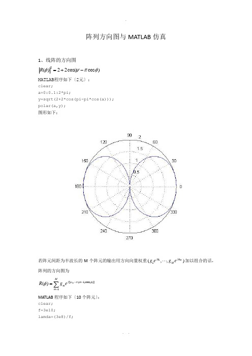
阵列方向图与MATLAB 仿真1、线阵的方向图2()22cos(cos )R φψπφ=+-MATLAB 程序如下〔2元〕:clear;a=0:0.1:2*pi;y=sqrt(2+2*cos(pi-pi*cos(a)));polar(a,y); 图形如下:若阵元间距为半波长的M 个阵元的输出用方向向量权重11(,,)M j j M g eg e φφ⋅⋅⋅加以组合的话,阵列的方向图为 [(1)cos()]1()m Mj m m m R g e ψπφφ--==∑MATLAB 程序如下〔10个阵元〕:clear;f=3e10;lamda=(3e8)/f;beta=2.*pi/lamda;n=10;t=0:0.01:2*pi;d=lamda/4;W=beta.*d.*cos(t);z1=((n/2).*W)-n/2*beta* d;z2=((1/2).*W)-1/2*beta* d;F1=sin(z1)./(n.*sin(z2));iK1=abs(F1) ;polar(t,K1);方向图如下:2、圆阵方向图程序如下:clc;clear all;close all;M = 16; % 行阵元数k = 0.8090; % k = r/lambdaDOA_theta = 90; % 方位角DOA_fi = 0; % 俯仰角% 形成方位角为theta,俯仰角位fi的波束的权值m = [0 : M-1];w = exp(-j*2*pi*k*cos(2*pi*m'/M-DOA_theta*pi/180)*cos(DOA_fi*pi/180));% w = exp(-j*2*pi*k*(cos(2*pi*m'/M)*cos(DOA_theta*pi/180)*cos(DOA_fi*pi/180)+sin(2*pi*m'/M)*si n(DOA_fi*pi/180))); % 竖直放置% w = chebwin(M, 20) .* w; % 行加切比雪夫权% 绘制水平面放置的均匀圆阵的方向图theta = linspace(0,180,360);fi = linspace(0,90,180);for i_theta = 1 : length(theta)for i_fi = 1 : length(fi)a = exp(-j*2*pi*k*cos(2*pi*m'/M-theta(i_theta)*pi/180)*cos(fi(i_fi)*pi/180));%a=exp(-j*2*pi*k*(cos(2*pi*m'/M)*cos(theta(i_theta)*pi/180)*cos(fi(i_fi)*pi/180)+sin(2*pi*m'/ M)*sin(fi(i_fi)*pi/180))); % 竖直放置Y(i_theta,i_fi) = w'*a;endendY= abs(Y); Y = Y/max(max(Y));Y = 20*log10(Y);% Y = (Y+20) .* ((Y+20)>0) - 20; % 切图Z = Y + 20;Z = Z .* (Z > 0);Y = Z - 20;figure; mesh(fi, theta, Y); view([66, 33]);title('水平放置时的均匀圆阵方向图');% title('竖面放置时的均匀圆阵方向图'); % 竖直放置axis([0 90 0 180 -20 0]);xlabel('俯仰角/(\circ)'); ylabel('方位角/(\circ)'); zlabel('P/dB');figure; contour(fi, theta, Y);方向图如下:3、平面阵方向图:clc;clear all;close all;Row_N = 16; % 行阵元数Col_N = 16; % 列阵元数k = 0.5; % k = d/lambdaDOA_theta = 90; % 方位角DOA_fi = 0; % 俯仰角% 形成方位角为theta,俯仰角位fi的波束的权值Row_n = [0 : Row_N-1]; Col_n = [0 : Col_N-1];W_Row = exp(-j*2*pi*k*Row_n'*cos(DOA_theta*pi/180)*cos(DOA_fi*pi/180)); W_Col = exp(-j*2*pi*k*Col_n'*sin(DOA_theta*pi/180)*cos(DOA_fi*pi/180)); % W_Col = exp(-j*2*pi*k*Col_n'*sin(DOA_fi*pi/180)); % 竖直放置W_Row = chebwin(Row_N, 20) .* W_Row; % 行加切比雪夫权W_Col = chebwin(Col_N, 30) .* W_Col; % 列加切比雪夫权W = kron(W_Row, W_Col); % 合成的权值N*N x 1% 绘制水平面放置的平面阵的方向图theta = linspace(0,180,180);fi = linspace(0,90,90);for i_theta = 1 : length(theta)for i_fi = 1 : length(fi)row_temp = exp(-j*2*pi*k*Row_n'*cos(theta(i_theta)*pi/180)*cos(fi(i_fi)*pi/180)); % 行导向矢量N x 1col_temp = exp(-j*2*pi*k*Col_n'*sin(theta(i_theta)*pi/180)*cos(fi(i_fi)*pi/180)); % 列导向矢量N x 1% col_temp = exp(-j*2*pi*k*Col_n'*sin(fi(i_fi)*pi/180)); % 竖直放置Y(i_theta,i_fi) = W'*kron(row_temp, col_temp); % 合成的导向矢量N*N x 1 endendY= abs(Y); Y = Y/max(max(Y));Y = 20*log10(Y);Y = (Y+60) .* ((Y+60)>0) - 60; % 切图% Z = Y + 60;% Z = Z .* (Z > 0);% Y = Z - 60;figure; mesh(fi, theta, Y); view([66, 33]);title('水平面放置时的面阵方向图');axis([0 90 0 180 -60 0]);xlabel('俯仰角/(\circ)'); ylabel('方位角(\circ)'); zlabel('P/dB');figure; contour(fi, theta, Y);方向图如下:4、CAPON方法波束形成MATLAB程序如下〔阵元16,信号源3,快拍数1024〕:clear alli=sqrt(-1);j=i;M=16;%均匀线阵列数目P=3;%信号源数目f0=10;f1=50;f2=100;%信号频率nn=1024;%快拍数angle1=-15;angle2=15;angle3=30;%the signal angleth=[angle1;angle2;angle3]';SN1=10;SN2=10;SN3=10;%信噪比sn=[SN1;SN2;SN3];degrad=pi/180;tt=0:.001:1024;x0=exp(-j*2*pi*f0*tt);%3个信号x0、x1、x2x1=exp(-j*2*pi*f1*tt); %x2=exp(-j*2*pi*f2*tt); %t=1:nn;S=[x0(t);x1(t);x2(t)];nr=randn(M,nn);ni=randn(M,nn);u=nr+j*ni;%复高斯白噪声Ps=S*S'./nn;%信号能量ps=diag(Ps);refp=2*10.^(sn/10);tmp=sqrt(refp./ps);S2=diag(tmp)*S;%加入噪声tmp=-j*pi*sin(th*degrad);tmp2=[0:M-1]';a2=tmp2*tmp;A=exp(a2);X=A*S2+.1*u;%接收到的信号Rxx=X*X'./nn;%相关矩阵invRxx=inv(Rxx);%搜寻信号th2=[-90:90]';tmp=-j*pi*sin(th2'*degrad);tmp2=[0:M-1]';a2=tmp2*tmp;A2=exp(a2);den=A2'*invRxx*A2;doa=1./den;semilogy(th2,doa,'r');title('spectrum'); xlabel('angle'); ylabel('spectrum'); axis([-90 90 1e1 1e5]); grid;。
MATLAB在天线方向图中的应用与研究
MATLAB在天线方向图中的应用与研究王曼珠1,张民1,崔红跃2(1.北京电子科技学院 通信工程系,北京100070;2.中国民用航空大学,天津300300)ª摘 要:以天线方向图函数为例,分析了对称阵子天线、阵列天线方向图函数F(H,U)随各参量变化的规律以及二维图形的特点,并讨论了直线天线阵(单向端射阵)的最大辐射方向和主瓣宽度随各参量变化的二维、三维图形特点。
借助M AT LAB的绘图功能,对各种天线的方向图函数的二维、三维图形进行研究,可以观察到天线辐射场在不同方向的辐射能量分布,直观清楚地表现出辐射方向图的特点。
关键词:天线;M AT LAB;辐射方向图中图分类号:TN820.1+2;TP391.77 文献标识码:A文章编号:1008-0686(2004)04-0024-04The Application and Study of Antenna Radiation Pattern Based on MATLABWANG Man-zhu1,ZHANG Zhe-min1,C UI Hong-yue2(1.Dep t.of Communication Eng ineer ing B eij ing E le ctronic S cience&T echnology I nstitute,B eij ing100070,China;2.Civ il A viation Unive rsity of China,T ianj ing300300,China)Abstract:This paper takes the antenna radiation pattern as an exam ple,and analy zes the rules of the function F(H,U)varg ing w ith the par am eters for the dipole and antenna ar rays r adiation pattern,as w ell as the characteristic of the tw o-dimensio nal fig ure.In addition,w e discuss the characteristics of the two and thr ee-dimensional fig ure when the max imum radiation and the width o f m ajo r lobe vary s w ith the param eters in the end-fire array.It introduces the w ay of plo tting co mplicated antenna directional r adiation pattern of two and three-dim ensional figure w ith the help of plo tting functions of MAT LAB,the radiating energy distribution of the antenna radiation field in different directions can be observed from r adiation pattern of the antenna,and the characteristic of the radiation pattern can be sho w n clearly.Keywords:antenna;M AT LA B;radiation pattern 天线的远区场分布是一组复杂的函数,分析不同天线的辐射场可从中得到该天线的各种重要性能参数。
阵列天线方向图的MATLAB实现
阵列天线方向图的MATLAB 实现课程名称:MATLAB程序设计与应用任课教师:周金柱班级:04091202姓名:黄文平学号:04091158成绩:阵列天线方向图的MATLAB 实现摘要:天线的方向性是指电磁场辐射在空间的分布规律,文章以阵列天线的方向性因子F(θ,φ)为主要研究对象来分析均匀和非均匀直线阵天线的方向性。
讨论了阵列天线方向图中主射方向和主瓣宽度随各参数变化的特点,借助M ATLAB绘制出天线方向性因子的二维和三维方向图,展示天线辐射场在空间的分布规律,表现辐射方向图的特点。
关键词:阵列天线;;方向图;MATLAB前言:天线是发射和接收电磁波的重要的无线电设备,没有天线也就没有无线电通信。
不同用途的天线要求其有不同的方向性,阵列天线以其较强的方向性和较高的增益在工程实际中被广泛应用。
因此,对阵列天线方向性分析在天线理论研究中占有重要地位。
阵列天线方向性主要由方向性因子F(θ,φ)表征,但F(θ,φ)在远区场是一组复杂的函数,如果对它的认识和分析仅停留在公式中各参数的讨论上,很难理解阵列天线辐射场的空间分布规律[ 1 ]。
MATLAB以其卓越的数值计算能力和强大的绘图功能,近年来被广泛应用在天线的分析和设计中。
借助MATLAB可以绘制出阵列天线的二维和三维方向图,直观地从方向图中看出主射方向和主瓣宽度随各参数的变化情况,加深对阵列天线辐射场分布规律的理解。
1 均匀直线阵方向图分析若天线阵中各个单元天线的类型和取向均相同,且以相等的间隔d 排列在一条直线上。
且各单元天线的电流振幅均为I,相位依次滞后同一数值琢,那么,这种天线阵称为均匀直线式天线阵,如图1 所示[ 2 ]:均匀直线阵归一化阵因子为[ 3 ]:Fn(θ,φ)是一个周期函数,所以除§= 0 时是阵因子的主瓣最大值外,§= ±2 mπ(m=1,2,...)都是主瓣最大值,这些重复的主瓣称为栅瓣,在实际应用中,通常希望出现一个主瓣,为避免出现栅瓣,必须把g限制在- 2π<§<2π范围内[ 4 ],其中k=λ/2π,即波数,n 表示阵元数目。
微波传输线三种工作状态分析的MATLAB实现
(一)主程序变量说明:输入变量:zo 传输线特性阻抗zl 传输线终端负载阻抗Er 传输线介电常数f 传输电磁波的频率由输入变量计算得出的变量:w 传输电磁波的数字角频率len 传输电磁波的相波长beita 相移常数gama 传输线个点反射系数复值gamal 传输线终端反射系数的模rou 驻波系数k 行波系数Zi 传输线各点输入阻抗的复值Ui 传输线各点输入电压的复值Uo 传输线各点输出电压的复值Uit 传输线各点输入电压的瞬时值Uot 传输线各点输出电压的瞬时值Ii 传输线各点输入电流的复值Io 传输线各点输出电流的复值Is 传输线各点合成电流的复值Us 传输线各点合成电压的复值Ist 传输线各点合成电流的瞬时值Ust 传输线各点合成电压的瞬时值ph 传输线各点合成电压的相位(二)主程序流程说明:本程序的界面中共有三个输入编辑框,三个输出编辑框和五个波形显示窗口,分别用来输入:传输线特性阻抗Z0、传输线终端负载阻抗Z L、传输的电磁波的频率f、传输线传输介质的相对介电常数εr;输出:传输线的终端反射系数ΓL、行波系数ρ、驻波系数K;具体的程序思路如下:1.由输入编辑框获得用户输入的Z0、Z L、f和εr;2.在“开始”按钮的callback函数中进行运算,并控制各个axis的显示;3.图形的动态显示由一个while循环实现,并由全局标记变量flag控制;4.在“停止”按钮的callback函数中令flag = 1,while循环跳出。
(三)程序运行效果1.行波演示中端接匹配负载zo = zl = 50Ω2.驻波演示1)终端短路zo = 50Ωzl = 02)终端开路zo = 50Ωzl = inf3)终端接纯电抗负载zo = 50Ωzl = X * j3.行驻波演示(四)主程序代码function varargout = StatusAnaly(varargin)%********************************************************%% Copyright (C), 2009-2012,Lyric %% FileName: StatusAnaly.m %% Author: Lyric %% Version: 1.0 %% Date: 2010-05-11 %%********************************************************%% STATUSANALY M-file for StatusAnaly.fig% STATUSANALY, by itself, creates a new STATUSANALY or raises the existing% singleton*.%% H = STATUSANALY returns the handle to a new STATUSANALY or the handle to % the existing singleton*.%% STATUSANALY('CALLBACK',hObject,eventData,handles,...) calls the local% function named CALLBACK in STATUSANALY.M with the given input arguments. %% STATUSANALY('Property','Value',...) creates a new STATUSANALY or raises the % existing singleton*. Starting from the left, property value pairs are% applied to the GUI before StatusAnaly_OpeningFcn gets called. An% unrecognized property name or invalid value makes property application% stop. All inputs are passed to StatusAnaly_OpeningFcn via varargin.%% *See GUI Options on GUIDE's Tools menu. Choose "GUI allows only one% instance to run (singleton)".%% See also: GUIDE, GUIDATA, GUIHANDLES% Edit the above text to modify the response to help StatusAnaly% Last Modified by GUIDE v2.5 11-May-2010 14:30:20% Begin initialization code - DO NOT EDITgui_Singleton = 1;gui_State = struct('gui_Name', mfilename, ...'gui_Singleton', gui_Singleton, ...'gui_OpeningFcn', @StatusAnaly_OpeningFcn, ...'gui_OutputFcn', @StatusAnaly_OutputFcn, ...'gui_LayoutFcn', [] , ...'gui_Callback', []);if nargin && ischar(varargin{1})gui_State.gui_Callback = str2func(varargin{1});endif nargout[varargout{1:nargout}] = gui_mainfcn(gui_State, varargin{:});elsegui_mainfcn(gui_State, varargin{:});end% End initialization code - DO NOT EDIT% --- Executes just before StatusAnaly is made visible.function StatusAnaly_OpeningFcn(hObject, eventdata, handles, varargin) % This function has no output args, see OutputFcn.% hObject handle to figure% eventdata reserved - to be defined in a future version of MATLAB% handles structure with handles and user data (see GUIDATA)% varargin command line arguments to StatusAnaly (see VARARGIN)% Choose default command line output for StatusAnalyhandles.output = hObject;% Update handles structureguidata(hObject, handles);% UIWAIT makes StatusAnaly wait for user response (see UIRESUME)% uiwait(handles.figure1);% --- Outputs from this function are returned to the command line.function varargout = StatusAnaly_OutputFcn(hObject, eventdata, handles)% varargout cell array for returning output args (see VARARGOUT);% hObject handle to figure% eventdata reserved - to be defined in a future version of MATLAB% handles structure with handles and user data (see GUIDATA)% Get default command line output from handles structurevarargout{1} = handles.output;function edit_zo_Callback(hObject, eventdata, handles)% hObject handle to edit_zo (see GCBO)% eventdata reserved - to be defined in a future version of MATLAB% handles structure with handles and user data (see GUIDATA)% Hints: get(hObject,'String') returns contents of edit_zo as text% str2double(get(hObject,'String')) returns contents of edit_zo as a double% --- Executes during object creation, after setting all properties.function edit_zo_CreateFcn(hObject, eventdata, handles)% hObject handle to edit_zo (see GCBO)% eventdata reserved - to be defined in a future version of MATLAB% handles empty - handles not created until after all CreateFcns called% Hint: edit controls usually have a white background on Windows.% See ISPC and COMPUTER.if ispc && isequal(get(hObject,'BackgroundColor'), get(0,'defaultUicontrolBackgroundColor'))set(hObject,'BackgroundColor','white');endfunction edit_zl_Callback(hObject, eventdata, handles)% hObject handle to edit_zl (see GCBO)% eventdata reserved - to be defined in a future version of MATLAB% handles structure with handles and user data (see GUIDATA)% Hints: get(hObject,'String') returns contents of edit_zl as text% str2double(get(hObject,'String')) returns contents of edit_zl as a double% --- Executes during object creation, after setting all properties.function edit_zl_CreateFcn(hObject, eventdata, handles)% hObject handle to edit_zl (see GCBO)% eventdata reserved - to be defined in a future version of MATLAB% handles empty - handles not created until after all CreateFcns called% Hint: edit controls usually have a white background on Windows.% See ISPC and COMPUTER.if ispc && isequal(get(hObject,'BackgroundColor'), get(0,'defaultUicontrolBackgroundColor'))set(hObject,'BackgroundColor','white');end% --- Executes on button press in btn_begin.function btn_begin_Callback(hObject, eventdata, handles)% hObject handle to btn_begin (see GCBO)% eventdata reserved - to be defined in a future version of MATLAB% handles structure with handles and user data (see GUIDATA)%获得传输线特性阻抗temp = get(handles.edit_zo, 'string');zo = str2num(temp);%获得传输线负载阻抗temp = get(handles.edit_zl, 'string');zl = str2num(temp);%获得传输介质相对介电常数temp = get(handles.edit_Er, 'string');Er = str2num(temp);%获得传输线上传播的电磁波频率temp = get(handles.edit_f, 'string');f = str2num(temp) * 1000000;w = 2 * pi * f;%获得相波长、相位常数len = GetLen(f, Er);L = 2 * len; %横坐标范围L为两倍的相波长beita = GetBeita(f, Er);z = linspace(0, L, 200);zn = z ./ len; %zn为相对于相波长len归一化的横坐标%获得反射系数[gamal, gama] = GetGama(zo, zl, beita, z);set(handles.edit_gama, 'string', num2str(abs(gamal)));%获得驻波系数rou = GetRou(gamal);set(handles.edit_rou, 'string', num2str(rou));%获得行波系数k = 1 / rou;set(handles.edit_k, 'string', num2str(k));t = 0;Ts = 0.06;fs = 4 * f;%标记变量,当flag = 1 时图像停止,当flag = 0 时图像继续运动global flagflag = 0;while flag == 0%获得传输线输入阻抗Zi = GetZi(zo, gama);%绘制传输线输入阻抗plot(handles.axes_zi, zn, abs(Zi));if max(abs(Zi)) > 500limzL = 0;limzH = 500;elseif (max(abs(Zi)) - min(abs(Zi))) < 1limzL = min(abs(Zi)) - 1;limzH = max(abs(Zi)) + 1;elselimzL = min(abs(Zi));limzH = max(abs(Zi));endaxis(handles.axes_zi, [0, max(zn), limzL, limzH]);title(handles.axes_zi, '输入电阻波形');xlabel(handles.axes_zi, 'z(lamda)');ylabel(handles.axes_zi, 'Zin(ohmic)');%获得传输线输入输出电压[Ui, Uo] = GetUio(beita, gama, z);[Uit, Uot] = GetUiot(Ui, Uo, f, t);%绘制传输线输入输出电压plot(handles.axes_u, zn, Uit, 'b', zn, Uot, 'r');axis(handles.axes_u, [0, max(zn), -1, 1]);title(handles.axes_u, '入射和反射电压波形');xlabel(handles.axes_u, 'z(lamda)');ylabel(handles.axes_u, 'Ui/Uo(V)');legend(handles.axes_u, 'Ui', 'Uo', 2);%获得传输线入射和反射电流[Ii, Io] = GetIio(Ui, zo, gama);%获得传输线合成电压、电流[Is, Us] = GetIUs(Ui, Uo, Ii, Io);[Ist, Ust] = GetIUst(Is, Us, f, t);%绘制传输线合成电压、电流plot(handles.axes_us, zn, Ust);limu = 1 + abs(gamal);axis(handles.axes_us, [0, max(zn), -limu, limu]);title(handles.axes_us, '合成电压波形');xlabel(handles.axes_us, 'z(lamda)');ylabel(handles.axes_us, 'Us(V)');plot(handles.axes_is, zn, Ist);limi = (1 + abs(gamal)) / zo;axis(handles.axes_is, [0, max(zn), -limi, limi]);title(handles.axes_is, '合成电流波形');xlabel(handles.axes_is, 'z(lamda)');ylabel(handles.axes_is, 'Is(A)');%获得并绘制电压相位ph = angle(Us .* exp(1i * 2 * pi * f /fs * t));plot(handles.axes_ph, zn, ph / pi);axis(handles.axes_ph, [0, max(zn), -1.1, 1.1]);title(handles.axes_ph, '合成电压相位波形');xlabel(handles.axes_ph, 'z(lamda)');ylabel(handles.axes_ph, 'thita(pi)');t = t + Ts;pause(Ts);end% --- Executes on button press in btn_stop.function btn_stop_Callback(hObject, eventdata, handles)% hObject handle to btn_stop (see GCBO)% eventdata reserved - to be defined in a future version of MATLAB% handles structure with handles and user data (see GUIDATA)global flagflag = 1;function edit_gama_Callback(hObject, eventdata, handles)% hObject handle to edit_gama (see GCBO)% eventdata reserved - to be defined in a future version of MATLAB% handles structure with handles and user data (see GUIDATA)% Hints: get(hObject,'String') returns contents of edit_gama as text% str2double(get(hObject,'String')) returns contents of edit_gama as a double% --- Executes during object creation, after setting all properties.function edit_gama_CreateFcn(hObject, eventdata, handles)% hObject handle to edit_gama (see GCBO)% eventdata reserved - to be defined in a future version of MATLAB% handles empty - handles not created until after all CreateFcns called% Hint: edit controls usually have a white background on Windows.% See ISPC and COMPUTER.if ispc && isequal(get(hObject,'BackgroundColor'), get(0,'defaultUicontrolBackgroundColor'))set(hObject,'BackgroundColor','white');endfunction edit_rou_Callback(hObject, eventdata, handles)% hObject handle to edit_rou (see GCBO)% eventdata reserved - to be defined in a future version of MATLAB% handles structure with handles and user data (see GUIDATA)% Hints: get(hObject,'String') returns contents of edit_rou as text% str2double(get(hObject,'String')) returns contents of edit_rou as a double% --- Executes during object creation, after setting all properties.function edit_rou_CreateFcn(hObject, eventdata, handles)% hObject handle to edit_rou (see GCBO)% eventdata reserved - to be defined in a future version of MATLAB% handles empty - handles not created until after all CreateFcns called% Hint: edit controls usually have a white background on Windows.% See ISPC and COMPUTER.if ispc && isequal(get(hObject,'BackgroundColor'), get(0,'defaultUicontrolBackgroundColor'))set(hObject,'BackgroundColor','white');endfunction edit_k_Callback(hObject, eventdata, handles)% hObject handle to edit_k (see GCBO)% eventdata reserved - to be defined in a future version of MATLAB% handles structure with handles and user data (see GUIDATA)% Hints: get(hObject,'String') returns contents of edit_k as text% str2double(get(hObject,'String')) returns contents of edit_k as a double% --- Executes during object creation, after setting all properties.function edit_k_CreateFcn(hObject, eventdata, handles)% hObject handle to edit_k (see GCBO)% eventdata reserved - to be defined in a future version of MATLAB% handles empty - handles not created until after all CreateFcns called% Hint: edit controls usually have a white background on Windows.% See ISPC and COMPUTER.if ispc && isequal(get(hObject,'BackgroundColor'), get(0,'defaultUicontrolBackgroundColor'))set(hObject,'BackgroundColor','white');endfunction edit_f_Callback(hObject, eventdata, handles)% hObject handle to edit_f (see GCBO)% eventdata reserved - to be defined in a future version of MATLAB% handles structure with handles and user data (see GUIDATA)% Hints: get(hObject,'String') returns contents of edit_f as text% str2double(get(hObject,'String')) returns contents of edit_f as a double% --- Executes during object creation, after setting all properties.function edit_f_CreateFcn(hObject, eventdata, handles)% hObject handle to edit_f (see GCBO)% eventdata reserved - to be defined in a future version of MATLAB% handles empty - handles not created until after all CreateFcns called% Hint: edit controls usually have a white background on Windows.% See ISPC and COMPUTER.if ispc && isequal(get(hObject,'BackgroundColor'), get(0,'defaultUicontrolBackgroundColor'))set(hObject,'BackgroundColor','white');endfunction edit_Er_Callback(hObject, eventdata, handles)% hObject handle to edit_Er (see GCBO)% eventdata reserved - to be defined in a future version of MATLAB% handles structure with handles and user data (see GUIDATA)% Hints: get(hObject,'String') returns contents of edit_Er as text% str2double(get(hObject,'String')) returns contents of edit_Er as a double% --- Executes during object creation, after setting all properties.function edit_Er_CreateFcn(hObject, eventdata, handles)% hObject handle to edit_Er (see GCBO)% eventdata reserved - to be defined in a future version of MATLAB% handles empty - handles not created until after all CreateFcns called% Hint: edit controls usually have a white background on Windows.% See ISPC and COMPUTER.if ispc && isequal(get(hObject,'BackgroundColor'), get(0,'defaultUicontrolBackgroundColor'))set(hObject,'BackgroundColor','white');end% --- Executes during object creation, after setting all properties.function axes_u_CreateFcn(hObject, eventdata, handles)% hObject handle to axes_u (see GCBO)% eventdata reserved - to be defined in a future version of MATLAB% handles empty - handles not created until after all CreateFcns called % Hint: place code in OpeningFcn to populate axes_u(五)子程序代码(按照在主程序中出现的顺序排列)function Len = GetLen(f, Er)%********************************************************%% Copyright (C), 2009-2012,Lyric %% FileName: GetLen.m %% Author: Lyric %% Version: 1.0 %% Date: 2010-05-11 %%********************************************************%% Function: GetLen% Description: 获得传输线上所传输的电磁波的相波长% Called By: StatusAnaly.m% Input: f 传输线中所传输电磁波的频率% Er 传输线中传输介质的相对介电常数% Return: Len 传输线中所传电磁波的相波长C = 300000000;Len = C / f / sqrt(Er);function Beita = GetBeita(f, Er)%********************************************************% % Copyright (C), 2009-2012,Lyric %% FileName: GetBeita.m %% Author: Lyric %% Version: 1.0 %% Date: 2010-05-11 %%********************************************************%% Function: GetBeita% Description: get the phase-shift constant 获得相移常数% Called By: StatusAnaly.m% Input: f the freqency of the wave propagated in the medium % Er the relative permittivity of the medium% Return: Beita the phase-shift constant of the wavepi = 3.1415926;%真空中的电磁波速度,单位:m/sC=300000000;%数字角频率W = 2 * pi * f;Beita = W * sqrt(Er) / C;function [GamaL, Gama] = GetGama(zo, zl, beita, z)%********************************************************% % Copyright (C), 2009-2012,Lyric %% FileName: GetGama.m % % Author: Lyric %% Version: 1.0 %% Date: 2010-05-11 %%********************************************************%% Function: GetGama% Description: get the reflection coefficient 获得反射系数% Called By: StatusAnaly.m% Input: zo the characteristic impedance of the transmission line % zl the load impedance of the transmission line% beita the phase-shift constant of the transmission line% z 相对于相波长归一化的横坐标% Return: GamaL 反射系数的模值% Gama 反射系数的复值if zl == infGamaL = 1;elseGamaL = (zl - zo) / (zl + zo);endGama = abs(GamaL) .* exp(-1i * 2 .* beita .* z);function Rou = GetRou(gamal)%********************************************************% % Copyright (C), 2009-2012,Lyric %% FileName: GetRou.m % % Author: Lyric %% Version: 1.0 %% Date: 2010-05-11 % %********************************************************%% Function: GetRou% Description: 获得传输线上的驻波系数% Called By: StatusAnaly.m% Input: gamal 传输线上的反射系数% Return: Rou 传输线上的驻波系数Gamal = abs(gamal);Rou = (1 + Gamal) / (1 - Gamal);function Zi = GetZi(zo, gama)%********************************************************% % Copyright (C), 2009-2012,Lyric %% FileName: GetZi.m % % Author: Lyric % % Version: 1.0 %% Date: 2010-05-11 %%********************************************************%% Function: GetZi% Description: 获得传输线上各点输入阻抗的复值% Called By: StatusAnaly.m% Input: zo 传输线的特性阻抗% gama 传输线上反射系数的复值% Return: Zi 传输线上各点输入阻抗的复值Zi = zo .* ((1 + gama) ./ (1 - gama));function [Ui, Uo] = GetUio(beita, gama, z)%********************************************************% % Copyright (C), 2009-2012,Lyric %% FileName: GetUio.m % % Author: Lyric % % Version: 1.0 %% Date: 2010-05-11 % %********************************************************%% Function: GetUio% Description: 获得输入输出电压的复值% Called By: StatusAnaly.m% Input: beita 传输线上电磁波的相移常数% gama 传输线上电磁波的反射系数% z 相对于相波长归一化的横坐标% Return: Ui 输入电压复值% Uo 输出电压复值% 假定输入电压模值为1U = 1;Ui = U * exp(1i * beita * z);Uo = Ui .* gama;function [Uit, Uot] = GetUiot(Ui, Uo, f, t)%********************************************************% % Copyright (C), 2009-2012,Lyric %% FileName: GetUiot.m % % Author: Lyric %% Version: 1.0 %% Date: 2010-05-11 % %********************************************************%% Function: GetUiot% Description: 获得输入输出电压瞬时值% Called By: StatusAnaly.m% Input: Ui 输入电压复值% Uo 输出电压复值% f 传输线上所传的电磁波的频率% t 当前时刻% Return: Uit 输入电压瞬时值% Uot 输出电压瞬时值%获得输入输出电压瞬时值fs = 4 * f;Uit = real(Ui .* exp(1i * 2 * pi * f / fs * t));Uot = real(Uo .* exp(1i * 2 * pi * f / fs * t));function [Ii, Io] = GetIio(Ui, zo, gama)%********************************************************% % Copyright (C), 2009-2012,Lyric %% FileName: GetIio.m %% Author: Lyric % % Version: 1.0 %% Date: 2010-05-11 % %********************************************************%% Function: GetIio% Description: 获得输入和输出电流的复值% Called By: StatusAnaly.m% Input: Ui 输入电压的复值% zo 传输线特征阻抗% gama 反射系数复值% Return: Ii 输入电流复值% Io 输出电流复值%获得输入输出电流复值Ii = Ui / zo;Io = - Ii .* gama;function [Is, Us] = GetIUs(Ui, Uo, Ii, Io)%********************************************************% % Copyright (C), 2009-2012,Lyric %% FileName: GetIUs.m % % Author: Lyric %% Version: 1.0 %% Date: 2010-05-11 % %********************************************************%% Function: GetIUs% Description: 获得合成电压电流复值% Called By: StatusAnaly.m% Input: Ui 输入电压复值% Uo 输出电压复值% Ii 输入电流复值% Io 输出电流复值% Return: Is 合成电流复值% Us 合成电压复值%获得合成电压电流复值%I2 = 1;%U2 = Zl * I2;%Us = U2 * cos(beita .* z) + 1i * Zo * I2 * sin(beita .* z);%Is = 1i * U2 /Zo * sin(beita .* z) + I2 * cos(beita .* z);Us = Ui + Uo;Is = Ii + Io;function [Ist, Ust] = GetIUst(Is, Us, f, t)%********************************************************%% Copyright (C), 2009-2012,Lyric %% FileName: GetIUst.m %% Author: Lyric %% Version: 1.0 %% Date: 2010-05-11 %%********************************************************%% Function: GetIUst% Description: 获得合成电压电流瞬时值% Called By: StatusAnaly.m% Input: Is 合成电流复值% Us 合成电压复值% f 电磁波频率% t 当前时间% Return: Ist 合成电流瞬时值% Ust 合成电压瞬时值%获得合成电压电流瞬时值fs = 4 * f;Ust = real(Us .* exp(1i * 2 * pi * f / fs * t));Ist = real(Is .* exp(1i * 2 * pi * f / fs * t));这是在下的大作业,新手编程,颇为拙劣,还望海涵。
手把手教你天线设计——用MATLAB仿真天线方向图

手把手教你天线设计——用MATLAB仿真天线方向图吴正琳天线是一种变换器,它把传输线上传播的导行波,变换成在无界媒介(通常是自由空间)中传播的电磁波,或者进行相反的变换。
在无线电设备中用来发射或接收电磁波的部件。
无线电通信、广播、电视、雷达、导航、电子对抗、遥感、射电天文等工程系统,凡是利用电磁波来传递信息的,都依靠天线来进行工作。
此外,在用电磁波传送能量方面,非信号的能量辐射也需要天线。
一般天线都具有可逆性,即同一副天线既可用作发射天线,也可用作接收天线。
同一天线作为发射或接收的基本特性参数是相同的。
这就是天线的互易定理。
天线的基本单元就是单元天线。
1、单元天线对称振子是一种经典的、迄今为止使用最广泛的天线,单个半波对称振子可简单地单独立地使用或用作为抛物面天线的馈源,也可采用多个半波对称振子组成天线阵。
两臂长度相等的振子叫做对称振子。
每臂长度为四分之一波长、全长为二分之一波长的振子,称半波对称振子。
对称振子是一种经典的、迄今为止使用最广泛的天线,单个半波对称振子可简单地单独立地使用或用作为抛物面天线的馈源,也可采用多个半波对称振子组成天线阵。
两臂长度相等的振子叫做对称振子。
每臂长度为四分之一波长、全长为二分之一波长的振子,称半波对称振子。
1.1用MATLAB画半波振子天线方向图主要是说明一下以下几点:1、在Matlab中的极坐标画图的方法:polar(theta,rho,LineSpec);theta:极坐标坐标系0-2*pirho:满足极坐标的方程LineSpec:画出线的颜色2、在方向图的过程中如果rho不用abs(f),在polar中只能画出正值。
也就是说这时的方向图只剩下一半。
3、半波振子天线方向图归一化方程:Matlab程序:clear alllam=1000;%波长k=2*pi./lam;L=lam/4;%天线臂长theta=0:pi/100:2*pi;f1=1./(1-cos(k*L));f2=(cos(k*L*cos(theta))-cos(k*L))./sin(theta);rho=f1*f2;polar(theta,abs(rho),'b');%极坐标系画图2、线性阵列天线2.1方向图乘积定理阵中第i 个天线单元在远区产生的电场强度为:2(,)ij i i i i ie E K If r πλθϕ-=式中,i K 为第i 个天线单元辐射场强的比例常数,i r 为第i 个天线单元至观察点的距离,(,)i f θϕ为第i 个天线单元的方向图函数,i I 为第i 个天线单元的激励电流,可以表示成为:Bji i i I a e φ-∆=式中,i a 为幅度加权系数,B φ∆为等间距线阵中,相邻单元之间的馈电相位差,亦称阵内相移值。
基于C++ Builder和Matlab实现天线方向图可视化软件的设计

: 兰: : : : : : ! 【
cos
图 2 4元 端 射 阵 的 二 维 、三 维方 向 图 ( 8滞 后 时)
( 三)c十B id r M ta 混合编程方法 + u Ie 与 a Ib
C + u ie +B i d r与 M t a a lb实现混合编程 的方法有 四种 : 调用 M t a n ie a I bE g n ,调用 M t a / + 数学 函数 库,使用 M to alb C + C acm
L: .2 2 为半波振子,最一化方 向性 函数 /
f c 1 o s
, = _ ( — I )
L: 为全波 振子 ,量一化方 向性 函数
【 收稿 日期 】2 1— 3 2 01 0— 3
工具 ,使用动态链接 库。本文使用 的是最后一种方法 。 通过 M t a a Ib自带 的 m c命令 ( 的 C m i e c 或 o p lr编译器 ) , 可 以把 由 M t a 编 写 的 m 函 数 文件 编 译 成 动 态 链接 库 a 1b
『 『一 / r
.
、
多个 控件 ,使用 它们来组建 应用程序非 常简单 。借助 于 c + +
B id r程序开发上 的强大优势 ,再携第 3方组件 资源的支 u e l 持 ,使 用 C +B id r开发应用程序变得轻松快 速而且功能 + ule
强大 。
墨
图1 1 4元 端射 阵 的
(l) d 1 。在 c +B i dr程序 中调用封装 的函数,实现 数值算 + u le
法 的运用。这种方法 只需在开发和发布 中包含其生成 的动态
库就可 以使程序脱 离 M t a a l b环境 。 本 文 程 序 的 使 用 环 境 为 M c o o t i d w X ir s f W n o s P P o e s o a P r f s i n l S 3系统 ,c + u le 编译器版 本为 6 0 + B id r ., Mta a lb版 本为 70 . 。在使用 中通过一个具体 的例 子来 说明程