BDD Circuit Optimization for Path Delay Fault-Testability
多源最短路算法

多源最短路算法多源最短路算法是指在图中找出多个起点到各个终点的最短路径的算法。
它是单源最短路算法的扩展,单源最短路算法只能求出一个起点到所有终点的最短路径,而多源最短路算法可以求出多个起点到所有终点的最短路径。
一、问题描述在一个有向带权图中,给定多个起点和终点,求每个起点到每个终点的最短路径。
二、常见算法1. Floyd算法Floyd算法是一种基于动态规划思想的多源最短路算法。
它通过不断地更新两个顶点之间的距离来得到任意两个顶点之间的最短路径。
Floyd 算法时间复杂度为O(n^3),空间复杂度为O(n^2)。
2. Dijkstra算法Dijkstra算法是一种单源最短路算法,但可以通过对每个起点运行一次Dijkstra算法来实现多源最短路。
Dijkstra算法时间复杂度为O(ElogV),空间复杂度为O(V)。
3. Bellman-Ford算法Bellman-Ford算法是一种解决带负权边图上单源最短路径问题的经典动态规划算法。
通过对每个起点运行一次Bellman-Ford算法来实现多源最短路。
Bellman-Ford算法时间复杂度为O(VE),空间复杂度为O(V)。
三、算法实现1. Floyd算法实现Floyd算法的核心思想是动态规划,即从i到j的最短路径可以通过i到k的最短路径和k到j的最短路径来得到。
因此,我们可以用一个二维数组dis[i][j]表示从i到j的最短路径长度,初始化为图中两点之间的距离,如果两点之间没有边相连,则距离为INF(无穷大)。
然后,我们用三重循环遍历所有顶点,每次更新dis[i][j]的值。
代码如下:```pythondef floyd(graph):n = len(graph)dis = [[graph[i][j] for j in range(n)] for i in range(n)]for k in range(n):for i in range(n):for j in range(n):if dis[i][k] != float('inf') and dis[k][j] != float('inf'):dis[i][j] = min(dis[i][j], dis[i][k] + dis[k][j])return dis```2. Dijkstra算法实现Dijkstra算法是一种贪心算法,它通过不断地选择当前起点到其他顶点中距离最小的顶点来更新最短路径。
工业机器人的路径规划算法考核试卷

A. A*算法
B. D*算法
C. Floyd算法
D. Bresenham算法
16.在路径规划中,以下哪种数据结构用于存储已访问的节点?()
A.开放列表
B.关闭列表
C.路径列表
D.邻接矩阵
17.关于工业机器人的路径规划,以下哪个描述是错误的?()
B. Dijkstra算法
C. D*算法
D. RRT算法
13.关于路径规划中的碰撞检测,以下哪种方法计算量相对较小?()
A.精确碰撞检测
B.粗略碰撞检测
C.迭代最近点法(ICP)
D.点到线段距离计算
14.以下哪项不是路径平滑处理的目的?()
A.降低路径长度
B.减少运动时间
C.减少能量消耗
D.增加路径上的拐点
3.用于评估路径规划算法性能的指标通常包括路径长度、规划时间和______。
4.在路径规划中,为了减少计算量,常用的空间划分技术有四叉树和______。
5.机器人路径规划中的碰撞检测可以通过______和基于几何的碰撞检测两种方法实现。
6.路径平滑处理的目的是为了减少路径的拐点,提高路径的______和可执行性。
A. A*算法
B. Dijkstra算法
C. Floyd算法
D. Bresenham算法
2.下列哪种算法不属于路径规划中的启发式搜索算法?()
A. A*算法
B. D*算法
C. IDA*算法
D. Breadth First Search算法
3.在A*算法中,H(n)代表什么?()
A.从起始点到当前点的代价
4.在工业机器人路径规划中,如何处理动态障碍物?请提出一种算法或策略,并解释其工作原理和有效性。
基于遗传算法优化的BDD描述的数字电路功能测试
自动化测试计算机测量与控制.2003.11(3) Computer Measurement &Control ・163・收稿日期:2002-06-12。
作者简介:梁泳(1973-),男,广西南宁市人,硕士生,主要从事数字电路故障诊断方向的研究。
梁述海(1950-),男,湖北省武汉市人,教授,主要从事舰船机舱自动化与计算机仿真方向的研究。
文章编号:1671-4598(2003)03-0163-02 中图分类号:TP274 文献标识码:A基于遗传算法优化的BDD 描述的数字电路功能测试梁 泳,梁述海,李雁飞(海军工程大学动力工程学院,湖北武汉 430033)摘要:针对数字电路的测试两大难点,采用二元判决图(BDD )表示数字电路模型,同时由BDD 生成测试矢量来完成数字电路的功能测试。
在由VHDL 描述完整电路功能的基础上用遗传算法对BDD 的规模进行压缩优化。
整个系统构成简单,自动化程度高,测试耗时少。
关键词:数字电路;遗传算法;功能测试;BDDFunctional T est of Digital Circuits withBDD Description B ased on the Optimization of G enetic AlgorithmsL IAN G Y ong ,L IAN G Shu 2hai ,L I Yan 2fei(College of Power Eng.,Naval Univ.of Engineering ,Wuhan 430033,China )Abstract :Aimed at the difficulty of digital circuits testing ,the BDD (binary decision diagram )is used to describe the model of digital circuit and produce the test vector to the functional test of digital circuit.G enetic algorithm (G A )compresses and opti 2mizes the scale of BDD based on the VHDL decrypting the full functions of the circuit under test.The testing system is simple ,highly automatic and time -used less.K ey w ords :digital circuits ;genetic algorithms ;functional test ;BDD1 引言作用。
[IT计算机]山东大学ACM模板_图论
![[IT计算机]山东大学ACM模板_图论](https://img.taocdn.com/s3/m/baa8c21502d8ce2f0066f5335a8102d276a26169.png)
图论1.最短路径 (4)1)Dijkstra之优雅stl (4)2)Dijkstra__模拟数组 (4)3)Dijkstra阵 (5)4)SPFA优化 (6)5)差分约束系统 (7)2.K短路 (7)1)Readme (7)2)K短路_无环_Astar (7)3)K短路_无环_Yen (10)4)K短路_无环_Yen_字典序 (12)5)K短路_有环_Astar (15)6)K短路_有环_Yen (17)7)次短路经&&路径数 (20)3.连通分支 (21)1)图论_SCC (21)2)2-sat (23)3)BCC (25)4.生成树 (27)1)Kruskal (27)2)Prim_MST是否唯一 (28)3)Prim阵 (29)4)度限制MST (30)5)次小生成树 (34)6)次小生成树_阵 (36)7)严格次小生成树 (37)8)K小生成树伪代码 (41)9)MST计数_连通性状压_NOI07 (41)10)曼哈顿MST (43)11)曼哈顿MST_基数排序 (46)12)生成树变MST_sgu206 (49)13)生成树计数 (52)14)最小生成树计数 (53)15)最小树形图 (56)16)图论_最小树形图_double_poj3壹64 (58)5.最大流 (60)1)Edmonds_Karp算法 (60)2)SAP邻接矩阵 (61)3)SAP模拟数组 (62)4)SAP_BFS (63)5)sgu壹85_AC(两条最短路径) (64)6)有上下界的最大流—数组模拟 (67)6.费用流 (69)1)费用流_SPFA_增广 (69)2)费用流_SPFA_消圈 (70)3)ZKW数组模拟 (72)7.割 (73)1)最大权闭合图 (73)2)最大密度子图 (73)3)二分图的最小点权覆盖 (74)4)二分图的最大点权独立集 (75)5)无向图最小割_Stoer-Wagner算法 (75)6)无向图最大割 (76)7)无向图最大割(壹6ms) (76)8.二分图 (78)1)二分图最大匹配Edmonds (78)2)必须边 (79)3)最小路径覆盖(路径不相交) (79)4)二分图最大匹配HK (80)5)KM算法_朴素_O(n4) (81)6)KM算法_slack_O(n3) (82)7)点BCC_二分判定_(2942圆桌骑士) (84)8)二分图多重匹配 (86)9)二分图判定 (88)10)最小路径覆盖(带权) (89)9.一般图匹配 (90)1)带花树_表 (90)2)带花树_阵 (93)10.各种回路 (96)1)CPP_无向图 (96)2)TSP_双调欧几里得 (97)3)哈密顿回路_dirac (98)4)哈密顿回路_竞赛图 (100)5)哈密顿路径_竞赛图 (102)6)哈密顿路径_最优&状压 (102)11.分治树 (104)1)分治树_路径不经过超过K个标记节点的最长路径 (104)2)分治树_路径和不超过K的点对数 (107)3)分治树_树链剖分_Count_hnoi壹036 (109)4)分治树_QTree壹_树链剖分 (113)5)分治树_POJ3237(QTree壹升级)_树链剖分 (117)6)分治树_QTree2_树链剖分 (122)7)Qtree3 (125)8)分治树_QTree3(2)_树链剖分 (128)9)分治树_QTree4_他人的 (130)10)分治树_QTree5_无代码 (135)12.经典问题 (135)1)欧拉回路_递归 (135)2)欧拉回路_非递归 (136)3)同构_树 (137)4)同构_无向图 (140)5)同构_有向图 (141)6)弦图_表 (143)7)弦图_阵 (147)8)最大团_朴素 (149)9)最大团_快速 (149)10)极大团 (150)11)havel定理 (151)12)Topological (151)13)LCA (152)14)LCA2RMQ (154)15)树中两点路径上最大-最小边_Tarjan扩展 (157)16)树上的最长路径 (160)17)floyd最小环 (161)18)支配集_树 (162)19)prufer编码_树的计数 (164)20)独立集_支配集_匹配 (165)21)最小截断 (168)最短路径Dijkstra之优雅stl#include <queue>using namespace std;#define maxn 壹000struct Dijkstra {typedef pair<int, int> T; //first: 权值,second: 索引vector<T> E[maxn]; //边int d[maxn]; //最短的路径int p[maxn]; //父节点priority_queue<T, vector<T>, greater<T> > q;void clearEdge() {for(int i = 0; i < maxn; i ++)E[i].clear();}void addEdge(int i, int j, int val) {E[i].push_back(T(val, j));}void dijkstra(int s) {memset(d, 壹27, sizeof(d));memset(p, 255, sizeof(p));while(!q.empty()) q.pop();int u, du, v, dv;d[s] = 0;p[s] = s;q.push(T(0, s));while (!q.empty()) {u = q.top().second;du = q.top().first;q.pop();if (d[u] != du) continue;for (vector<T>::iterator it=E[u].begin();it!=E[u].end(); it++){ v = it->second;dv = du + it->first;if (d[v] > dv) {d[v] = dv;p[v] = u;q.push(T(dv, v));}}}}};Dijkstra__模拟数组typedef pair<int,int> T;struct Nod {int b, val, next;void init(int b, int val, int next) {th(b); th(val); th(next);}};struct Dijkstra {Nod buf[maxm]; int len; //资源int E[maxn], n; //图int d[maxn]; //最短距离void init(int n) {th(n);memset(E, 255, sizeof(E));len = 0;}void addEdge(int a, int b, int val) {buf[len].init(b, val, E[a]);E[a] = len ++;}void solve(int s) {static priority_queue<T, vector<T>, greater<T> > q;while(!q.empty()) q.pop();memset(d, 63, sizeof(d));d[s] = 0;q.push(T(0, s));int u, du, v, dv;while(!q.empty()) {u = q.top().second;du = q.top().first;q.pop();if(du != d[u]) continue;for(int i = E[u]; i != -壹; i = buf[i].next) {v = buf[i].b;dv = du + buf[i].val;if(dv < d[v]) {d[v] = dv;q.push(T(dv, v));}}}}};Dijkstra阵//Dijkstra邻接矩阵,不用heap!#define maxn 壹壹0const int inf = 0x3f3f3f3f;struct Dijkstra {int E[maxn][maxn], n; //图,须手动传入!int d[maxn], p[maxn]; //最短路径,父亲void init(int n) {this->n = n;memset(E, 63, sizeof(E));}void solve(int s) {static bool vis[maxn];memset(vis, 0, sizeof(vis));memset(d, 63, sizeof(d));memset(p, 255, sizeof(p));d[s] = 0;while(壹) {int u = -壹;for(int i = 0; i < n; i ++) {if(!vis[i] && (u==-壹||d[i]<d[u])) {u = i;}}if(u == -壹 || d[u]==inf) break;vis[u] = true;for(int v = 0; v < n; v ++) {if(d[u]+E[u][v] < d[v]) {d[v] = d[u]+E[u][v];p[v] = u;}}}}} dij;SPFA优化/*** 以下程序加上了vis优化,但没有加slf和lll优化(似乎效果不是很明显)* 下面是这两个优化的教程,不难实现----------------------------------SPFA的两个优化该日志由 zkw 发表于 2009-02-壹3 09:03:06SPFA 与堆优化的 Dijkstra 的速度之争不是一天两天了,不过从这次 USACO 月赛题来看,SPFA 用在分层图上会比较慢。
欧拉回路构造算法
欧拉回路构造算法全文共四篇示例,供读者参考第一篇示例:欧拉回路是图论中的一个重要概念,在一幅图中指的是一条包含图中每一条边且经过每一条边仅一次的闭合路径。
欧拉回路构造算法是指寻找一条欧拉回路的方法,即将给定的图转化为满足欧拉回路性质的路径。
欧拉回路构造算法有多种,其中最为经典和常用的算法是Fleury 算法和Hierholzer算法。
Fleury算法是一种基于贪心思想的算法,其基本思路是每次选择一条不是桥的边,通过DFS搜索来构造欧拉回路。
具体步骤如下:1. 从图中任选一个顶点作为起点。
2. 找到可以走的一条不是桥的边,并走向该边所连接的顶点。
3. 如果该边是割边,则在走完该边后,必须选择一条不是割边的边继续前进。
4. 重复步骤2和步骤3,直到不能走为止。
Fleury算法的时间复杂度为O(E^2),其中E为图中的边数。
Hierholzer算法是另一种求解欧拉回路的经典算法,其基本思想是通过遍历所有的边来构造欧拉回路。
具体步骤如下:1. 从图中任意一个顶点开始,选择一条边进行遍历。
2. 如果走到某个节点时无法继续行走,则回退到之前分叉点重新选择一条边继续遍历。
3. 直到遍历完所有的边,形成一个闭合回路即为欧拉回路。
欧拉回路构造算法的应用十分广泛,例如在网络设计、图像处理、数据压缩等领域都有着重要的作用。
通过欧拉回路构造算法,我们可以快速有效地找到一条经过所有边的闭合路径,从而解决一系列实际问题。
欧拉回路构造算法是解决图论中欧拉回路问题的重要工具。
不同的算法适用于不同的情况,可以根据具体问题的要求选择合适的算法。
通过学习和了解欧拉回路构造算法,我们可以更好地运用图论知识解决实际问题,提高问题解决的效率和准确性。
希望本文对读者有所帮助,欢迎大家进一步深入学习和探讨。
第二篇示例:欧拉回路构造算法是图论中一种重要的算法,用于寻找图中存在的欧拉回路。
欧拉回路是指一条包含所有边且不重复经过任何边的闭合路径。
在很多实际应用中,欧拉回路是一个非常有用的概念,比如在电子电路的布线设计、网络路由、以及城市旅行等领域都有很多应用。
改进遗传算法在含DG配电网重构中的应用

2020年第39卷第10期传感器与微系统(Transducer and Microsyslem Technologies)153{应用技术'DOI:10.13873/J.1000-9787(2020)10-0153-04改进遗传算法在含DG配电网重构中的应用金亦舟,张莉萍,武鹏,牛启帆,沈依婷(上海工程技术大学电子电气工程学院,上海201620)摘要:计及分布式电源(DC)出力和负荷不确定性对配电网的影响,提岀一种适用于不确定性配电网重构的改进遗传算法。
首先,基于DG出力概率模型,给出考虑多种不确定性的供电能力机会约束模型,建立了考虑供电能力机会约束条件的配电网重构模型;然后,改进遗传算法中生成初始种群与交叉操作的方式,使其适用于所建配电网重构模型;最后,使用改进遗传算法求解配电网重构模型,给出基于蒙特卡罗模拟的随机机会约束检验方法。
IEEE33节点算例的计算结果表明,本文方法能计及DG出力和负荷的不确定性,所得方案可满足设定的供电能力,提升配电网重构方案的抗风险能力。
关键词:配电网重构;改进遗传算法;供电能力;分布式电源;机会约束规划中图分类号:TM727文献标识码:A文章编号:1000-9787(2020)10-0153-04Application of improved GA in distribution networkreconfiguration with DGJIN Yizhou,ZHANG Liping,WU Peng,NIU Qifan,SHEN Yiting(School of Electronic and Electrical Engineering,Shanghai University of Engineering Science,Shanghai201620,China) Abstract:The impact of distributed generation(DG)access on distribution network is taken into account,animproved genetic algorithm for uncertain distribution network reconfiguration is proposed・Firstly,based on DGoutput probability model,a power supply capability index opportunity constraint model considering uncertainty ispresented,and the distribution network reconfiguration model considering chance constrained condition isestablished;then, the initial population generation and crossover operation of genetic algorithm is improved to makeit suitable for the uncertain distribution network reconfiguration model.Finally,a simulation method for calculatingthe chance constrained of power supply capability index is presented.The33ode example shows that the methodis able to take the uncertainty of DG output and distribution network load into account on the basis of traditionalgenetic algorithm,The reconfiguration scheme can meet the index of power supply capability and improve the anti・risk capability of the reconfiguration scheme.Keywords:distribution network reconfiguration;improved genetic algorithm;power supply capability index;distributed generation(DG);chance constrained programming0引言配电网重构是一种根据系统实时运行状况,通过优化网络拓扑来提高网架运行效率和电能质量的重要手段。
2020年第43卷总目次

Ⅲ
船用锅炉汽包水位内模滑模控制………………………………………………… 段蒙蒙ꎬ甘辉兵 ( 3. 83 )
三峡升船机变频器 IGBT 路故障诊断 ……………………… 孟令琦ꎬ高 岚ꎬ李 然ꎬ朱汉华 ( 3. 89 )
定航线下考虑 ECA 的船舶航速多目标优化模型 …………… 甘浪雄ꎬ卢天赋ꎬ郑元洲ꎬ束亚清 ( 3. 15 )
改进二阶灰色极限学习机在船舶运动预报中的应用………… 孙 珽ꎬ徐东星ꎬ苌占星ꎬ叶 进 ( 3. 20 )
Ⅱ
规则约束下基于深度强化学习的船舶避碰方法
………………………………… 周双林ꎬ杨 星ꎬ刘克中ꎬ熊 勇ꎬ吴晓烈ꎬ刘炯炯ꎬ王伟强 ( 3. 27 )
船用起重机吊索张力建模与计算机数值仿真 ………………………… 郑民民ꎬ张秀风ꎬ王任大 ( 4. 94 )
约束规划求解自动化集装箱码头轨道吊调度 ………………………… 丁 一ꎬ田 亮ꎬ林国龙 ( 4. 99 )
航海气象与环保
162 kW 柴油机排气海水脱硫性能
基于模糊 ̄粒子群算法的舰船主锅炉燃烧控制 ……… 毛世聪ꎬ汤旭晶ꎬ汪 恬ꎬ李 军ꎬ袁成清 ( 1. 88 )
多能源集成控制的船舶用微电网系统频率优化……………… 张智华ꎬ李胜永ꎬ季本山ꎬ赵 建 ( 1. 95 )
基于特征模型的疏浚过程中泥浆浓度控制系统设计………… 朱师伦ꎬ高 岚ꎬ徐合力ꎬ潘成广 ( 2. 74 )
基于卷积神经网络的航标图像同态滤波去雾 …………………………………………… 陈遵科 ( 4. 84 )
船用北斗导航系统终端定位性能的检测验证 …………………………………………… 吴晓明 ( 4. 89 )
改进鲸鱼优化算法在机器人路径规划中的应用
lengthꎬ and the number of turning points of the algorithms givenꎬ which verifies the effectiveness
第44 卷 第8 期
2023 年 8 月
东 北 大 学 学 报 ( 自 然 科 学 版 )
Journal of Northeastern University( Natural Science)
Vo l. 44ꎬNo. 8
Aug. 2 0 2 3
doi: 10. 12068 / j. issn. 1005 - 3026. 2023. 08. 001
evolutionꎬ the global exploration ability and convergence speed are improved. Meanwhileꎬ by
introducing the PSO algorithm with strong optimization ̄seeking ability into the exploitation stage
始解ꎬ增强了算法跳出局部最优的能力. 最后ꎬ将 PSO - AWOA 算法应用到的栅格地图仿真环境中进行机器
人最佳路径求解. 通过对比给定算法的耗时、规划路径长度以及拐点数ꎬ结果表明ꎬ提出的 PSO - AWOA 算法
在优化精度和收敛速度上优于文中给定的其他算法ꎬ验证了改进算法的有效性.
关 键 词: 混合优化算法ꎻ粒子群优化ꎻ鲸鱼优化算法ꎻ自适应权重ꎻ路径规划
里程计和全方位自动导引车的外部传感器(AGV的)同时校准
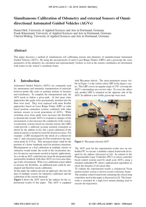
with Mecanum wheels. The most prominent sensor visible in Figure 1 is the yellow safety LRF in the figure’s center. This LRF covers an angular range of 270◦ covering the AGV’s surrounding area on two sides. To cover the others side another LRF is mounted on the opposite side of the AGV. In addition a not visible gyroscope were used.
2.1
Calibration of multiple Laser Range Finder (LRF)
Calibration of multiple LRF or Light Detection and Ranging (LIDAR) sensors was introduced in [2]. This paper discusses the on-line calibration of two LIDAR sensors by using natural features in an outdoor scenario. Through utilizing the described process the sensor data of both sensors is kept aligned. The vehicle used in this paper is a conventional automobile with an Ackermann steering instead of an omnidirectional AGV. Furthermore both scanners are setup in a manner, that create vertical scan lines while the setup discussed in this paper uses scanners creating horizontal scan lines.
c++最短路径算法和充电问题
在计算机科学领域,最短路径算法是一类重要的算法,可以帮助我们找到图中两个顶点之间的最短路径。
而在现实生活中,充电问题也是一个备受关注的话题,特别是在智能手机、电动车等设备普及的今天,人们对于如何高效地给这些设备充电也越来越感兴趣。
C++是一种高效、灵活的编程语言,它有着丰富的库函数和工具,使得我们可以很方便地实现最短路径算法和解决充电问题。
在本文中,我们将从简到繁地探讨C++最短路径算法和充电问题,并对它们进行全面评估。
一、最短路径算法1. Dijkstra算法Dijkstra算法是一种经典的最短路径算法,它可以在带权重的图中找到单源最短路径。
在C++语言中,我们可以使用STL库中的priority_queue和vector来实现Dijkstra算法,通过使用最小堆来维护当前离源点最近的节点,同时动态更新节点的最短路径值。
2. Floyd-Warshall算法Floyd-Warshall算法是一种多源最短路径算法,它可以有效地处理带权重的有向图或无向图。
在C++中,我们可以使用二维数组来表示节点之间的距离关系,并通过动态规划的方式逐步更新最短路径值。
3. Bellman-Ford算法Bellman-Ford算法是一种解决带有负权边的最短路径问题的算法,它可以检测出图中是否存在负权回路,并找出最短路径。
在C++中,我们可以使用数组来表示节点的最短路径值,并通过对每条边进行多次松弛操作来逐步逼近最短路径值。
二、充电问题在现代社会,充电问题已经成为了人们生活中不可或缺的一部分。
无论是手机、电动车还是笔记本电脑,它们都需要不断地充电以保持正常使用。
在这样的背景下,如何高效地解决充电问题就显得尤为重要。
1. 充电桩的分布充电桩的分布对充电问题有着重要的影响。
在城市中,如果充电桩分布得当,可以有效地解决人们出行中的充电问题,提高出行的便捷性。
在C++中,我们可以使用图论算法来模拟充电桩的分布,找到最佳的布局方案。
中国邮递员问题

6
5
3 4
v5 4
v9
3 v8 4
v1
9
v4
4
v7
v3 5 v2 5
v1
2
v6 4
3
6
4
v5
4
v9
3 v8
4
9
v4
4
v7
运筹学
判定标准1: 在最优邮递路线上,图中的每一条 边至多有一条重复边。
判定标准2 : 在最优邮递路线上,图中每一个 圈的重复边总权小于或等于该圈总权的一半。
例8.12 求解下图所示网络的中国邮路问题,图中数 字为该边的长。
v3 2 v6 4 v9
5
3
v2
6 v5
5
4
3
4
v8
4
v1
9
v4
4
v7
v3 2 v6 4 v9
A
C
D
B
二、 奇偶点图上作业法 (1)找出图G中的所有的奇顶点,把它们两两配 成对,而每对奇点之间必有一条通路,把这条通路 上的所有边作为重复边追加到图中去,这样得到的 新连通图必无奇点。 (2)如果边e=(u,v)上的重复边多于一条,则 可从重复边中去掉偶数条,使得其重复边至多为一 条,图中的顶点仍全部都是偶顶点。 (3)检查图中的每一个圈,如果每一个圈的重 复边的总长不大于该圈总长的一半,则已经求得最 优方案。如果存在一个圈,重复边的总长大于该圈 总长的一半时,则将这个圈中的重复边去掉,再将 该圈中原来没有重复边的各边加上重复边,其它各 圈的边不变,返回步骤(2)。
运筹学
中国邮递员问题
一、 欧拉回路与道路 定义8.18 连通图G中,若存在一条道路,经过每 边一次且仅一次,则称这条路为欧拉道路。若存 在一条回路,经过每边一次且仅一次,则称这条 回路为欧拉回路。 具有欧拉回路的图称为欧拉图。 定理8.7 一个多重连通图G是欧拉图的充分必要 条件是G中无奇点。 推论 一个多重连通图G有欧拉道路的充分必要 条件是G有且仅有两个奇点。
巡查机器人路径规划算法与应用综述

巡查机器人路径规划算法与应用综述目录一、内容描述 (2)1.1 背景与意义 (3)1.2 国内外研究现状 (4)1.3 研究内容与方法 (6)二、巡查机器人路径规划算法概述 (6)2.1 路径规划的定义与重要性 (8)2.2 常见的路径规划算法 (9)三、基于遗传算法的路径规划 (10)3.1 遗传算法原理简介 (12)3.2 遗传算法在路径规划中的应用 (13)3.3 改进遗传算法的策略 (14)四、基于蚁群算法的路径规划 (16)4.1 蚂蚁系统算法(AS) (17)4.2 最大最小蚂蚁系统(MMAS) (18)4.3 蚁群优化算法在路径规划中的应用及特点 (19)五、基于粒子群算法的路径规划 (21)5.1 粒子群算法(PSO)简介 (22)5.2 PSO在路径规划中的应用 (23)5.3 改进粒子群算法的策略 (24)六、基于其他智能算法的路径规划 (25)6.1 模拟退火算法(SA) (26)6.2 神经网络算法 (27)6.3 混合智能算法在路径规划中的应用 (29)七、路径规划在实际应用中的挑战与解决方案 (31)7.1 实际应用场景分析 (32)7.2 面临的主要挑战 (33)7.3 应对策略与技术手段 (35)八、总结与展望 (36)8.1 研究成果总结 (37)8.2 存在的不足与局限性 (38)8.3 对未来研究的展望 (39)一、内容描述随着现代社会对高效、智能、安全监控需求的日益增长,巡查机器人在城市管理、公共安全、工业生产等多个领域的应用逐渐普及。
为了实现高效、准确的路线规划,路径规划算法在其中发挥着至关重要的作用。
本文将对巡查机器人路径规划算法及其在实际应用中的研究进展进行综述,旨在为相关领域的研究提供有益的参考。
巡查机器人路径规划算法的研究涵盖了多个学科领域,包括人工智能、计算机视觉、机器人学等。
随着深度学习技术的快速发展,基于深度学习的路径规划算法在图像识别、传感器融合等方面取得了显著成果。
c++迪杰斯特拉算法

c++迪杰斯特拉算法迪杰斯特拉算法是一种用于计算最短路径的算法,它是由荷兰计算机科学家艾兹格·迪杰斯特拉(Edsger W. Dijkstra)在20世纪50年代中期所发明的。
在许多实际应用中,最短路径问题是一件非常重要的事情。
比如说,在地图上规划路径、网络中找寻最短路径等等。
迪杰斯特拉算法在实际应用中有着广泛的用途。
迪杰斯特拉算法能够计算出从指定起点出发到其他各个顶点的最短路径。
在计算过程中,算法会维护一个集合S,集合S中的顶点表示已经求得的最短路径。
算法还会维护一个集合Q,集合Q中的顶点表示还未求得最短路径的顶点。
算法会在集合Q的顶点中寻找到起点到该顶点路径长度最短的那个顶点,并将该顶点加入到集合S中。
迪杰斯特拉算法的基本思想就是贪心策略。
算法会选择当前数据中距离起点最近的顶点k,并将k加入到S中。
然后,算法会检查所有从k出发的边,更新起点到其他顶点的最短路径,如果发现了一条比原来更短的路径,就更新路径长度和前驱顶点。
下面是C++实现Dijkstra算法的代码:```#include <iostream>#include <vector>#include <queue>#include <cstring>using namespace std;struct node {int v, w;};const int maxn = 1e6 + 7;const int inf = 0x3f3f3f3f;bool vis[maxn];int dist[maxn];vector<node> G[maxn];这段代码中,我们用了一个vector来存储所有的边,用一个优先队列来维护当前距离起点最短的未访问的顶点。
我们用vis来记录每个顶点是否已经处理过。
因为我们要更新起点到所有顶点的最短路径,所以我们需要遍历所有的边。
运行以上代码,我们可以输入一个n个顶点和m条边的图,以及起点s和终点t,算法就可以输出s到t的最短路径。
金属年代项目 EQ-73 均衡器说明说明书

W W W .G O L D E N A G E P R O J E C T .C O MIEQ-73INTRODUCTIONCongratulations on choosing the Golden Age Project EQ-73 Equalizer!The class-A circuit used in the EQ-73 is similar to the eq section in the classical 1073 module, without the high pass filter. Additional frequencies have been added and the mid frequency band uses two inductors, the higher value of the second one is used for the two lowest frequencies, 160 Hz and 240 Hz, to achieve a suit-able response.The sound character is warm, punchy, sweet and musical. These classic characteristics have been heard on countless recordings through the years and it is a versatile sound that works very well on most sound sources and in most genres. The essence of this sound is now available at a surprisingly low cost, making it available to nearly everyone.The EQ-73 has stepped frequency controls that offers a wide selection of frequencies from 20 Hz to 24 kHz. The Low and High frequency bands are shelving and the mid frequency band is of the bell type. The control range is +/-15 dB for the two lower bands and +/- 18dB for the high frequency band. There are separate bypass switches for all three bands.The EQ-73 cannot be used as a standalone EQ. It is made to be used together with one of our PRE-73 models that has an Insert jack.Combining a PRE-73 and an EQ-73, and using a UNITE rack kit to mount them together, one will get a 19-inch 1073-style unit at a low cost and with a great sound! FEATURES- Vintage Style electronics. No intergrated circuits in the signal path - 3-band with a dual inductor based mid frequency band - Stepped frequency selection- A wide selection of frequencies from 20 Hz to 24 kHz - Control range up to +/- 18 dB - Separate Bypass switches for each band - Tantalum capacitors in the signal path- Made to be used together with one of our PRE-73 models with an Insert jack - TRS jack for in-and output connection, the nominal working level is around 18 dBu - Selectable ground lift switch- External power supply to avoid interaction with the audio circuits - Great sound that suits most sound sources and genres - A solid build quality that will last many years of normal useCIRCUIT DESCRIPTIONThe main signal path in the EQ-73 con-sists of two gain stages that uses threetransitors each and a few resistors andcapacitors. So, all in all, the completesignal chain only contains six active ele-ments. Compare that to the big numberof transistors that are usually used inone single integrated circuit! The filter circuits uses additional passive components.The first gain stage handles the LF and HF bands and the second gain stage handles the MF band. By designing the EQ-73 to be used with a PRE-73 with an Insert jack, the unit does not have to be fitted with an input and output stage.The MF band uses two inductors and capacitors for a classicLC-style eq circuit. The first inductor has a several taps to achieve suitable Q-values (ie, the shape of the curve) for the different mid frequencies from 350 Hz to 10 kHz. The second inductor has a higher value and are used for the two lowest mid frequencies, 160 Hz and 240 Hz.MODERN VERSUS OLDIt is true that there are some great IC´s available today that achieves very low levels of static and dynamic distortion.The simple circuits that the EQ-73 uses, cannot match the low distor-tion specifications of modern IC´s.It is the distortion components that imparts a sound characterto the audio signal and, if the distortion components are of the right sort, this is a good thing since it makes the recorded voice or instrument sound “better”, more musical, more pleasing to the ear. This is one reason why vintage style units are so popular today.This is not to suggest that modern, transparent sounding audio circuits is a bad thing, sometimes they are prefered over colored ones. It´s all about taste and it depends on the genre. For most modern music styles, color and character is definitely a good thing.And doesn´t it feel good to use audio components built according to the old, minimalistic approach where one can follow the signal from one discrete component to another?USING THE EQ-73Using an equalizer is not rocket science. Here are some points though to help you getting the maximum out of the EQ-73:- Connect the cable from the power supply to the AC 24V connec-tor at the back of the EQ-73. Power on the unit with the front panel POWER switch.- Connect the supplied stereo TRS cable between the back panel TRS jack and the Insert jack of the PRE-73.- The EQ-73 will now be inserted in the signal path of the PRE-73. If you are using the EQ-73 together with a PRE-73 DLX, you must engage the INSERT switch to activate the EQ-73.- The best way to learn how to set the controls of the EQ-73 is to experiment with different settings on different sound sources. There are a number of frequencies added to the original design, expanding the possibilities for soundshaping.- The LF and HF bands are of the shelving type, ie, it affects all frequencies below (LF) and above (HF) the selected frequency. The eq action starts gradually above (LF) or below (HF) the selectedfrequency and increases up to the maximum boost or cut. The MF has a bell curve, ie, a cut or boost centered around the resonance frequency.- By engaging the OUT switches, the eq action of each band can be easily removed for quick comparions between eq and no eq. Using the INSERT switch in the PRE-73 DLX, one can instantly bypass the complete EQ-73 from the signal path.- There is a Ground Lift switch on the back panel. It should nor-mally be in the OUT position. If the EQ-73 is mounted in a UNITE rack kit together a PRE-73 and / or mounted in a rack where other units are also mounted, ground loops can give rise to problems. Try engaging the Ground Lift switch which will lift the circuit board ground from the cabinet of the EQ-73.PLEASE NOTE:- The maximum boost and cut varies somewhat with the selected frequency.- Inserting the EQ-73 in a PRE-73 will result in a small gain change.- Clicks can arise when the controls are operated, especially on the HF band. This is normal and a consequence of the used circuit design.- The inductors and the filter circuits in the EQ-73 are sensitive to electromagnetic fields. If you have a problem with hum or noise, try moving the unit to another physical location in your studio. One situation where this problem is most likely to show up is if the EQ-73 is mounted above or close to a unit that contain a power supply with a mains transformer.WARRANTYThe EQ-73 is built to last. But as in any electronic device, compo-nents can break down.There is a fast blow fuse located inside the unit. If the unit dies, please check this fues. If it has blown, replace it with a new one. You can also try with another 24V AC adaptor if you have one avail-able.If this doesn´t help, or if the unit has another problem, it will need repair and you should then contact the reseller where you bought the unit.The warranty period is decided by the Distributor for your country. The Distributor will support Golden Age Project resellers and end users with repairs and spare parts.REGISTRATIONYou are welcome to register your unit at our website:---------------------------I would like to thank you for chosing the EQ-73!I hope it will serve you well and that it will help you inmaking many great sounding recordings.Yours,Bo MedinCreate music– Be happy!W W W.G O L D E N A G E P R O J E C T.C O M。
秃鹫优化算法python
秃鹫优化算法python(实用版)目录1.秃鹫优化算法的概念与原理2.秃鹫优化算法的应用实例3.秃鹫优化算法的优点与局限性4.秃鹫优化算法的 Python 实现5.未来研究方向与展望正文一、秃鹫优化算法的概念与原理秃鹫优化算法(Condor Optimization Algorithm, COA)是一种受秃鹫觅食行为启发的优化算法。
秃鹫在觅食过程中,会根据环境因素和食物分布,选择最有利的路径进行搜索。
COA 模仿了秃鹫的这种行为,将其应用到优化问题中,通过搜索最优解来解决实际问题。
COA 的主要原理包括:1.随机初始化:算法开始时,随机生成一组初始解,用于后续的搜索过程。
2.位置更新:每个个体在搜索过程中,会根据自身的位置和全局最优位置,更新自己的位置,以逼近最优解。
3.食物分布更新:在搜索过程中,食物的分布会影响个体的移动策略。
当个体找到食物时,会根据食物分布的更新规则,调整食物的位置,从而影响后续的搜索过程。
二、秃鹫优化算法的应用实例秃鹫优化算法在很多领域都有应用,例如:1.机器学习:在机器学习中,COA 可以用于解决特征选择、参数优化等问题。
2.信号处理:在信号处理领域,COA 可以用于信号调制、滤波器设计等问题。
3.控制工程:在控制工程中,COA 可以用于控制器设计、优化等问题。
三、秃鹫优化算法的优点与局限性秃鹫优化算法的优点包括:1.寻优能力强:COA 具有很强的全局搜索能力,能够找到全局最优解。
2.收敛速度快:COA 的收敛速度较快,能够在较短时间内找到满意解。
3.适应性强:COA 适应性强,能够应对不同问题的特点,进行有效搜索。
然而,COA 也存在一些局限性,例如:1.参数设置复杂:COA 的参数设置较为复杂,需要根据问题特点进行调整。
2.算法稳定性较低:COA 的算法稳定性较低,容易出现早熟现象,影响算法性能。
归结原则
最短路算法的应用研究作者:张丽赟指导教师:王骁力摘要:最短路问题是网络理论中应用最广泛的问题之一,Dijkstra算法[1]是求解最短路问题的一种经典算法。
但这种算法不能有效解决含负权的最短路问题,并且算法复杂性比较大。
现在含负权值的最短路问题已有了解决的方法[2]。
同时结合求最小树的Kruskal算法和破圈运算,也有了求一类最短路问题的简单算法[3],并且该算法复杂性比递推法要好。
结合实例讨论这些算法在运输问题,含负权值的最短路问题以及线路优化问题等方面的应用。
关键词:有向图;最短路;算法;应用最短路问题是网络分析中的一个基本问题,同时也是图及网络理论中的重要问题,许多实际问题都可以转化为最短路问题或者把最短路问题作为其子问题,如设备更新、管道铺设、厂区布局、线路安排等,因此最短路可以直接用于解决实际问题,也可以作为一个基本工具,用于解决其他的优化问题。
运用并突破已有理论知识,寻找新的简单有效的方法,对于解决经济管理问题、运输线路优化等问题都有很重要的意义。
最短路的一般算法--Dijkstra算法[1]是最经典的一种方法,该方法也已十分的详尽,但算法的复杂度比较大,并且不能用来解决含负权的最短路问题。
结合求最小树的Kruskal算法和破圈运算,可以给出一类最短路问题的简单算法,运用图论、动态规划等方法也可以解决某些最短路问题。
现在的研究热点就是找出新的最短路算法来更加有效、更加全面的解决经济管理、线路优化、运输问题等实际问题。
含负权的最短路问题很常见,因此本文讨论了有效解决含负权的最短路问题的新算法[2]。
结合求最小树的Kruskal算法和破圈运算,可以得到求解一类最短路问题的简单算法[3],该方法在算法复杂性上比Dijkstra算法要好。
探究新算法的目的常常是用来解决实际问题的,因此在给出具体算法后,相应给出具体事例来运用给出的新算法,从而也可以验证算法的有效性。
1预备知识1.1 有向图一个图是由一些点及一些点之间的连线(不带箭头或带箭头)所组成的,把带箭头的连线称为弧。
一个高效BDD的简洁实现
一个高效BDD的简洁实现苏开乐;吕关锋;宋炯【期刊名称】《计算机学报》【年(卷),期】2014(37)9【摘要】二叉判定图BDD作为一种表示和操作布尔函数的数据结构,被广泛地应用在模型检测、系统验证等领域.在最坏情况下,BDD的空间规模是指数级的,因此为了设计和实现一个高效BDD包,研究者们做了大量技术性工作,同时涌现出多个高效BDD包.为了节省空间和提高运算速度,这些BDD包的实现都限定了一个较小的变量个数上限(不超过2^(16)),然而这种限定同时也限制了BDD包的适用性.为了突破这种限制,文中给出了一个高效的BDD包实现,该包在采纳了经典BDD包高效实现技术的同时,使用了内存分片分配、轻量级垃圾回收等技术.这些技术使得BDD包在保持高性能的情况下,将可处理的变量规模提高到2^(32),与现有BDD包的处理规模2^(16)相比,大大提高了BDD包的适用性.实验证明其性能非常接近可获得的最快的2^(16)变量规模的BDD包——CUDD.【总页数】6页(P2021-2026)【关键词】二叉判定图;布尔函数;内存分配【作者】苏开乐;吕关锋;宋炯【作者单位】浙江师范大学数理信息工程学院,浙江金华312004;清华大学清华-阿姆斯特丹逻辑学联合研究中心,北京100084;北京工业大学计算机学院,北京100022【正文语种】中文【中图分类】TP301【相关文献】1.一个简洁高效的Ad Hoc移动自组网络仿真工具 [J], 付才;催永泉;彭冰;李俊2.一个高效犅犇犇的简洁实现 [J], 苏开乐;吕关锋;宋炯3.高效制备BDD单体新方法探究 [J], 张鹏兵;高文婷;刘晨旭;周鹏鑫4.打造一个简洁高效的课堂 [J], 耿玉兰5.Hibernate:一个简洁高效的ORM框架 [J], nickheudecker; 郑涛因版权原因,仅展示原文概要,查看原文内容请购买。
用递归BDD(二元决策图)技术分析因果图

用递归BDD(二元决策图)技术分析因果图严晓;王洪春【摘要】故障树是以系统最不希望发生的顶事件为目标,通过分析找出导致顶上事件发生的全部因素;在故障树分析中,二元决策图(简称BDD)是最有效的方法之一,由于故障树和因果图都是用图形表示因果关系,两者具有很多相似性,而BDD在故障树中有广泛的应用;通过研究表明:在一定条件下,故障树和因果图之间可以互相转化,因此可以分析BDD的原理,并将BDD技术用来分析因果图.【期刊名称】《重庆工商大学学报(自然科学版)》【年(卷),期】2015(032)008【总页数】4页(P34-37)【关键词】故障树;BDD;因果图【作者】严晓;王洪春【作者单位】重庆师范大学数学学院,重庆401331;重庆师范大学数学学院,重庆401331【正文语种】中文【中图分类】O141.41**通讯作者:王洪春(1967-),男,四川大竹人,教授,博士,从事人工智能、因果图和故障诊断研究.E-mail:*********************.cn故障树是一种以系统最不希望发生的顶事件为目标,通过对可能导致顶事件发生的中间事件和底事件进行分析,在一般情况下,事件分为两种状态,正常或者是故障,在传统分析故障树中,一般通过求故障树的最小割集,对故障树进行分析,然而对于复杂的故障树,求最小割集比较困难,为了克服这种缺陷,引入了二元决策图[1],把故障树转化成二元决策图进行分析研究,然后自上而下遍历二元决策图,能够得到最小割集,在二元决策图转化的过程中,要先对故障树进行简化,对简化后的故障树的基本事件进行排序[2],从而对故障树进行定性和定量分析。
而因果图是从信度网发展起来的,通过事件连接成一个网状结构来反映事件之间的关系,通过研究表明,在一定条件下因果图和故障树之间可以相互转化,因此BDD也可以用于因果图中。
将故障树转化为BDD的方法,最早是由Rauzy提出的,并在转化过程中提出了一种ite结构(If-then-Else),它是基于shannon分解提出来的,ite(x,y,z)表示如果x成立,则成立,否则,z成立,数学表达式为ite(x,y,z) = xy+z。
- 1、下载文档前请自行甄别文档内容的完整性,平台不提供额外的编辑、内容补充、找答案等附加服务。
- 2、"仅部分预览"的文档,不可在线预览部分如存在完整性等问题,可反馈申请退款(可完整预览的文档不适用该条件!)。
- 3、如文档侵犯您的权益,请联系客服反馈,我们会尽快为您处理(人工客服工作时间:9:00-18:30)。
BDD Circuit Optimization for Path Delay Fault-TestabilityGörschwin Fey Junhao Shi Rolf DrechslerInstitute of Computer ScienceUniversity of Bremen28359Bremen,Germanyfey,junhao,drechsle@informatik.uni-bremen.deAbstractThe complexity of integrated circuits is rapidly growing. This leads to more and more time and money spent on the test of these circuits.Besides minimizing the logic needed for a given function the testability of the resulting circuit becomes a major issue during synthesis.One way to syn-thesize a circuit for a given function is to directly convert the Binary Decision Diagram(BDD)of that function into a circuit.It is known that optimizations of the BDD transfer to the derived circuit.Therefore in this paper we evaluate dif-ferent optimization techniques for BDDs based on variable reordering with respect to the path delay fault testability of the resulting circuit.We show an optimization strategy that allows to compromise during synthesis between logic size and testability.1.IntroductionSize and complexity of physically producible circuits steadily increase.This establishes the need to consider the aspect of testing for physical faults already during synthesis since otherwise this task becomes too time consuming.Binary Decision Diagrams(BDDs)are often used in VLSI CAD systems for efficient representation and manip-ulation of Boolean functions[5,6].In particular they have been studied in logic synthesis,since they allow to consider aspects of technology mapping[11].It is a well-known synthesis approach to map the BDD to a multiplexor cir-cuit.Testability of these circuits with respect to the Path Delay Fault Model(PDFM)has been investigated in[2,3] and[1]already.The PDFM is a very powerful fault model that allows to detect static and dynamic faults.The major drawback is the large number of paths that have to be tested. Solutions based on test points or synthesis transformations have been proposed in[12,14],but e.g.test point insertion requires additional hardware.Here,we use techniques to minimize the BDD.Thus,the optimization can be carried out earlier in the synthesis pro-cess by using symbolic methods.Our methods are based on variable reordering.Sifting is a well-known and fre-quently used reordering heuristic to minimize the number of nodes in a BDD[15].But we apply sifting to minimize with respect to the number of paths,the average path length or a combined measure incorporating number of nodes and paths.This optimizations of the BDD directly transfer to the circuit.Experiments show the feasibility of the approach.The structure of the paper is as follows:In Section 2BDDs and BDD circuits are defined and the PDFM is briefly reviewed.The minimization of BDDs is described in Section3.Experimental results are given in Section4, followed by the conclusions in Section5.2.Preliminaries2.1.Binary Decision Diagrams and CircuitsAs is well-known,each Boolean functioncan be represented by a BDD,i.e.a directed acyclic graph where a Shannon decomposition is carried out in each node.A BDD is called ordered if each variable is encountered at most once on each path from the root to a terminal node and if the variables are encountered in the same order on all such paths.A BDD is called reduced if it does neither contain isomorphic sub-BDDs nor vertices with both edges pointing to the same node.In the following,only reduced, ordered BDDs are considered and for briefness these graphs are called BDDs.BDDs are a canonical representation,i.e. for each Boolean function the BDD can be uniquely deter-mined.Furthermore,for functions represented by BDDs efficient manipulations are possible[5].A combinational circuit implementing a function can be retrieved from a BDD by replacing each node of the function with a multiplexer(see Figure1).This multiplexer can be implemented by basic gates over the standard library consisting of primary input and output ports,the2-input/1-output AND-and OR-gate and the1-input/1-output inverter NOT.Mapxif1fvf1sFigure1.Mapping a BDD to a circuit(a)Order(b)Figure2.BDDs of with respect to two variable ordersDefinition1.The size of a circuit is given by the number of gates it contains.Definition2.The depth of a circuit is the maximal number of gates on a path from an input to an output.2.2.Path Delay Fault ModelIn this paper we consider a dynamic fault model,i.e. the Path-Delay Fault Model(PDFM)[18].In the PDFM it is checked whether the propagation delays of all physical paths in a given combinational circuit are less than the sys-tem clock interval.To this end a transition,i.e.a change in the value of a signal,has to be propagated from pri-mary inputs to primary outputs.A transition(rising,falling)propagates along a path,if a se-quence of transitions occurs at the nodes,such that occurs as a result of.Definition3.A path has a Path Delay Fault(PDF),if the actual propagation delay of a(rising or falling)transition along the path exceeds the system clock interval.For the detection of a path delay fault a pair of patterns is required:The initialization vector is applied and all signals of the circuit are allowed to stabilize;then the propagation vector is applied and after the system clock interval the outputs of the circuit are controlled.Two tests for each physical path have to be carried out,since a check is done for rising and falling transitions.Definition4.A two-pattern test is called a robust test for a path delay fault(RPDF test)on a path,if it detects that fault independently of all other delays in the circuit and all other delay faults not located on the path.For a detailed discussion of the PDFM see[13].3.Minimizing the BDDsThe variable order of a BDD has a major influence on the number of its nodes.But to decide,if the number of nodes of a given BDD can be improved by variable reordering,is NP-complete[4].Therefore heuristics are used to minimize BDDs of non-trivial functions.One well-known heuristic is sifting[15]:A variable is chosen and moved to any position of the variable order based on exchanging adjacent variables.Then it isfixed at the best position(i.e.where the smallest BDD results),af-terwards another variable is chosen.No variable is chosen twice during this process.This heuristic can be used to min-imize a BDD with respect to other goals than the number of nodes by changing the objective function that measures the size.We consider four objective functions:1.Number of paths:2.Number of nodes:3.Average path length:4.Weighted sum of the number of paths and the numberof nodes:Number of paths An efficient algorithm to carry out sift-ing with respect to the number of paths was introduced in[9].Paths from roots to terminals in the BDD correspond to paths in the circuit.Therefore minimizing the number of paths in the BDDs leads to a smaller number of possibly erroneous paths in the circuit.By this,less test patterns are needed to test the resulting circuit.Number of nodes The change of the number of nodes can efficiently be calculated during sifting.Therefore thisobjective function leads to a fast minimization algorithm.Since a multiplexor corresponds to each node in the BDD, the size in terms of logic elements in the circuit is mini-mized by this function.Average path length Let be the number of paths with length and the total number of paths,then the average length of paths in the BDD is given by:#in#lits#paths71581071 alu260.8%41171410 clip582.1%35159384 frg1367.3%133198672Then the minimization was carried out andfinally the BDD-circuit was written(for more details see[2]).The number of literals needed for a circuit was determined using SIS [17],also the number of physical paths in the circuit and the path delay fault coverage were determined.In all of the following tables the notations of Section3are used to de-note objective functions and sizes.Table1shows characteristics of each circuit.Besides the number of primary inputs and outputs the number of liter-als needed after optimization by’script.rugged’from SIS is listed.Column’PDFC’gives the path delay fault coverage of the optimized circuit,i.e.the percentage of paths that can be covered by a RPDF test.For this coverage large varia-tions can be observed,in one case even less than1%of all paths can be tested(’alu2’).Next,Table2states the statistics on the BDDs that have been minimized with respect to the different objective func-tions.In case of the weighted objective function both parameters and were set to.The lowest number of paths for each circuit is printed bold.The minimization of a BDD with respect to one crite-rion does not always lead to the best result with respect to this criterion,e.g.’5xp1’turns out to have the least num-ber of nodes when minimized with respect to paths.This is due to the heuristic minimization algorithms:The objective function influences which parts of the search space are con-sidered.The average path length does not vary too much for the different objective ing it as the only optimization criterion can lead to large BDDs in terms of number of nodes.Much better results are produced when applying the weighted objective function,which often leads to the optimum for and within the four strategies.Es-pecially remarkable is’count’.Here leads to a BDD that has by far less nodes than in all other cases and also the number of paths is the smallest.Finally,Table3gives the data for the circuits derived from the BDDs.Here again,SIS was used to count the number of literals for the circuit.SIS was also used to prop-agate constants into the gates of the circuit using the com-mand’sweep’.This can result in differently sized circuits for same sized BDDs(e.g.’5xp1’for methods and). In general the BDD smallest in the number of nodes leads to the smallest circuit.One of the objective functions and always led to the circuit with the least number of physical paths.Espe-cially remarkable are the results for’i5’,where the num-ber of physical paths is reduced by a factor of12.The ob-jective function compared to method always lead to less physical paths while the size of the circuit on average dropped.In comparison to SIS in some cases(’5xp1’,’alu2’) a significant improvement in the number of paths and inTable2.BDD-statisticsObj.func.Circ.44 4.4218051 4.401611957.595301717.44506145 6.90785185 6.6361675 6.73626117 6.734282178.0913172537.1835211811.8675919410.57349135 6.608008482 6.00738#lits#paths PDFC#lits#paths PDFC5xp182.1%17225682.6%131218 alu285.9%62481481.4%598773 b965.2%364122863.0%390934 clip72.6%35796972.8%260648 count94.0%831216379.6%221624 frg165.9%399113577.4%320529 i568.9%10221167164.1%330975PDFC was gained,for’5xp1’even the size decreased.Op-posed to the large variations of the PDFC obtained for op-timized circuits from SIS,the PDFC was never below50% for any of the BDD circuits.5.Conclusions and Future WorkDifferent objective functions for BDD minimization were evaluated with respect to testability of the resulting BDD circuits.It was shown that the reduction of the num-ber of paths in the BDD can significantly reduce the num-ber of test patterns needed to test the circuit with respect to the PDFM.An adjustable objective function was used to take more than one goal during synthesis into account and thereby to compromise e.g.between size and number of test patterns needed.The major drawback of the current synthesis approach is the drop in the path delay fault coverage for some circuits. Therefore it is focus of current work to combine the pro-posed technique with the one from[7].In[7]MUX-circuits are synthesized that are guaranteed to be100%testable un-der the PDFM and the Stuck-at Fault Model at the cost of one additional input.References[1]P.Ashar,S.Devadas,and K.Keutzer.Path-delay-fault testa-bility properties of multiplexor-based networks.INTEGRA-TION,the VLSI Jour.,15(1):1–23,1993.[2] B.Becker.Synthesis for testability:Binary decision di-agrams.In Symp.on Theoretical Aspects of Comp.Sci-ence,volume577of LNCS,pages501–512.Springer Verlag, 1992.[3] B.Becker.Testing with decision diagrams.INTEGRATION,the VLSI Jour.,26:5–20,1998.[4] B.Bollig and I.Wegener.Improving the variable ordering ofOBDDs is NP-complete.IEEE Trans.on Comp.,45(9):993–1002,1996.[5]R.Bryant.Graph-based algorithms for Boolean functionmanipulation.IEEE Trans.on Comp.,35(8):677–691,1986.[6]R.Bryant.Binary decision diagrams and beyond:Enabelingtechniques for formal verification.In Int’l Conf.on CAD, pages236–243,1995.[7]R.Drechsler,J.Shi,and G.Fey.MuTaTe:An efficient de-sign for testability technique for multiplexor based circuits.In Great Lakes Symp.VLSI,2003.[8] E.Dubrova and ler.On disjoint covers and ROBDDsize.In Pacific Rim Conference on Communications,Com-puters and Signal Processing,pages162–164,1999.[9]G.Fey and R.Drechsler.Minimizing the number of pathsin BDDs.In Symposium on Integrated Circuits and System Design,pages359–364,2002.[10]G.Fey and R.Drechsler.Utilizing BDDs for disjoint SOPminimization.In Midwest Symposium on Circuits and Sys-tems,volume2,pages306–309,2002.[11]W.Günther and R.Drechsler.ACTion:Combining logicsynthesis and technology mapping for MUX based FPGAs.Journal of Systems Architecture,46(14):1321–1334,2000.[12] A.Kristi´c and K.-T.Cheng.Resynthesis of combinationalcircuits for path count reduction and for path delay fault testability.Jour.of Electronic Testing:Theory and Appli-cations,11:43–54,1997.[13]I.Pomeranz and S.Reddy.Delay fault models for VLSIcircuits.INTEGRATION,the VLSI Jour.,26:21–40,1998.[14]I.Pomeranz and S.M.Reddy.Design-for-testability for pathdelay faults in combinational circuits using test points.IEEE Trans.on CAD,17:333–343,1998.[15]R.Rudell.Dynamic variable ordering for ordered binary de-cision diagrams.In Int’l Conf.on CAD,pages42–47,1993.[16] C.Scholl,R.Drechsler,and B.Becker.Functional simula-tion using binary decision diagrams.In Int’l Conf.on CAD, pages8–12,1997.[17] E.Sentovich,K.Singh,vagno,C.Moon,R.Mur-gai,A.Saldanha,H.Savoj,P.Stephan,R.Brayton,andA.Sangiovanni-Vincentelli.SIS:A system for sequentialcircuit synthesis.Technical report,University of Berkeley, 1992.[18]G.Smith.Model for delay faults based upon paths.In Int’lTest Conf.,pages342–349,1985.。